Machine Learning & Signals Learning

C Solutions

Answer of exercise 1.1 Hint: substitute \(Y=aX+b\) into Eq. (1.17).

Answer of exercise 1.2 

\begin{align*} p[k\ge 4] &= 1 - p[k<4] \\ &= 1- \bigl ( p[k=1] + p[k=2] +p[k=3]\bigr ) \\ &= 1- \left (\frac {4}{7} + \frac {2}{7} + \frac {1}{8}\right )= \frac {1}{56} \end{align*}

Answer of exercise 1.3 Count the number of outcomes obtained for each possible outcome of the random experiment, and normalize by the total number of experiments.

N = 1e6;      % number of random experiments
x = randi(6,[1 N]);
y = randi(6,[1 N]);
z = x + y;
empirical_cdf = sum(z == (1:12)',2)/N;
bar(empirical_cdf)

Answer of exercise 1.4 The outcomes of the coin tosses follow a binomial distribution, where the number of successes \(k\) equals the number of tosses \(n\),

\[ X\sim \mathrm {Bin}(n,1/2)\Rightarrow p = p_X[k=n] =\dbinom {n}{n}p^n(1-p)^{n-n} = \left (\frac {1}{2}\right )^n \]

Method A: the outcome of repeating the experiment follows a binomial distribution, where the probability of a run of ones in each experiment is \(p\) from the previous part. After \(N\) experiments, the probability of one or more successes is the complement of the probability of zero successes, \(p_Y[0]\),

\begin{equation*} Y\sim \mathrm {Bin}(N,p)\Rightarrow p_2 = 1-p_Y[0] = 1- \left (1-p\right )^{N} = 1- \left (1-\left (\frac {1}{2}\right )^n\right )^{N} \end{equation*}

Method B: the probability of a single experiment outcome without a run of \(n\) ones is \(1-\left (\frac {1}{2}\right )^n\).

The probability of \(N\) experiment outcomes without a run of ones is \(\left (1-\left (\frac {1}{2}\right )^n\right )^N\). Of course, the final answer is identical.

\begin{equation*} p_2= 1- \left (1-\left (\frac {1}{2}\right )^{10}\right )^{2^{10}} = 0.632 \end{equation*}

Answer of exercise 1.5 

\begin{align*} X\sim \mathrm {Bin}(n=10^3,p=10^{-3})&,\quad p_X[0] = \binom {n}{0}p^0(1-p)^{n} \approx 0.37\\ X\sim \mathrm {Bin}(n=10^3,p=10^{-3})&,\quad p_X[1] = \binom {n}{1}p^1(1-p)^{n-1} \approx 0.37\\ X\sim \mathrm {Bin}(n=10^3,p=10^{-3})&,\quad \Pr (X\ge 3) = 1 - F_X(2) = 1 - p_X[0] - p_X[1] - p_X[2] \approx 0.08 \end{align*}

Answer of exercise 1.6 Define:

• • \(p\): the probability that a bit arrives erroneous (Error).

• • \(1-p\): the probability that a bit arrives correct (Correct).

Transmission without repetition (2 bits). In a transmission of 2 bits, an error is defined as the case in which at least one bit is erroneous. We compute this using the complementary event: the case in which there is no error at all (both bits are correct).

The probability that both bits are correct:

\[ \Pr (\text {correct message}) = (1-p) \cdot (1-p) = (1-p)^2 \]

The error probability is the complement to 1:

\begin{align*} \Pr (\text {error}) &= 1 - \Pr (\text {correct message}) = 1 - (1-p)^2\\ &= 1 - (1 - 2p + p^2) = 2p - p^2 \end{align*}

Completely correct transmission (4 bits). For the transmission to be received perfectly, all 4 bits (the 2 originals plus the 2 repetitions) must arrive without error. Since the bit errors are independent:

\[ \Pr (\text {perfect transmission}) = (1-p) \cdot (1-p) \cdot (1-p) \cdot (1-p) = (1-p)^4 \]

Undetected error with repetition (4 bits). Denote the transmission as \(M_1 M_2\), where \(M_1\) is the first pair and \(M_2\) is the repetition. An undetected error occurs when \(M_1 = M_2\) (the receiver accepts the transmission), but the value differs from the original value. This happens when exactly the same error occurs in both pairs.

Consider the possible types of errors in a block of 2 bits:

• • Error in the first bit only: the probability is \(p(1-p)\).

• • Error in the second bit only: the probability is \((1-p)p\).

• • Error in both bits: the probability is \(p \cdot p = p^2\).

For the error to go undetected, it must occur in both \(M_1\) and \(M_2\):

• 1. error in the first bit in both: \([p(1-p)] \times [p(1-p)] = p^2(1-p)^2\)

• 2. error in the second bit in both: \([(1-p)p] \times [(1-p)p] = p^2(1-p)^2\)

• 3. error in both bits in both: \([p^2] \times [p^2] = p^4\)

Summing the probabilities:

\[ \Pr (\text {undetected error}) = 2 \cdot p^2(1-p)^2 + p^4 = 2p^2(1-p)^2 + p^4 \]

Answer of exercise 1.7 (a, f)

Answer of exercise 1.8 

\begin{align*} X&\sim \mathrm {Geo}\left (p=\frac {1}{36}\right )\\ F_X(9)&= 1 - (1-p)^9\\ \Pr (X \ge 10) &= 1 - \Pr (X\le 9) = 1 - F_X(9)\\ & = \left (1-\frac {1}{36}\right )^9 = \left (\frac {35}{36}\right )^9\\ &=\frac {78815638671875}{101559956668416}\approx 0.776 \end{align*} Another approach, by computing the probability of 0 “successes” out of 9,

\begin{align*} X&\sim \mathrm {Bin}\left (9,\frac {1}{36}\right )\\ p_X[0] &= \binom {9}{0}p^0(1-p)^{9} = \left (\frac {35}{36}\right )^9 \end{align*} Parts (b) and (c),

\begin{align*} X&\sim \mathrm {Bin}\left (10,\frac {1}{36}\right )\\ p_X[0] &=\binom {10}{0}\left (\frac {1}{36}\right )^0\left (1-\frac {1}{36}\right )^{10}\approx 0.754493\\ \Pr (X\ge 1)& = 1 - F_X(0) = 1-p_X[0]\\ &= 1-\left (1-p\right )^n\\ &=1-\left (\frac {35}{36}\right )^{10}\approx 0.2455\\ p_X[1] &= \binom {10}{1}p^1(1-p)^{n-1} = 10\left (\frac {1}{36}\right )\left (1-\frac {1}{36}\right )^9\\ &= \frac {10}{36}\left (\frac {35}{36}\right )^9 \approx 0.21557 \end{align*}

Answer of exercise 2.1 

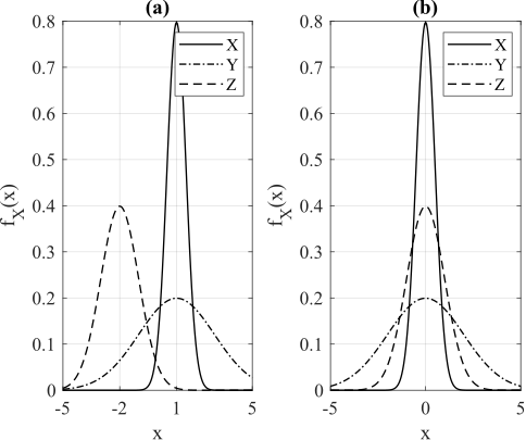
• (a) \(\mu _X = \mu _Y = 1, \mu _Z = -2\)

• (b) \(\sigma _X < \sigma _Z < \sigma _Y\)

The figure below shows the functions \(f_X(x)\) whose CDFs \(F_X(x) = \int _{- \infty }^x f_X(x)\,dx\) were shown in the question. In figure (a) the original functions \(f_X(x)\) are shown, and in figure (b) they are normalized to \(\mu _X = \mu _Y = \mu _Z = 0\).

Answer of exercise 2.2 The sum of independent Gaussian variables is Gaussian, so only its two parameters are needed. The expectation is additive, and so is the variance because the experiments are independent,

\begin{align*} \E [Y] &= 200\,\E [X_i] = 100, \\ \Var [Y] &= 200\,\Var [X_i] = \frac {200}{4} = 50 \end{align*} The interval is symmetric about the expectation, so the two tails are equal and the Q-function gives

\begin{align*} \Pr (90\le Y\le 110) &= \Pr (Y \ge 90)-\Pr (Y \ge 110)\\ &= Q\!\Bigl (\tfrac {90-100}{\sqrt {50}}\Bigr ) - Q\!\Bigl (\tfrac {110-100}{\sqrt {50}}\Bigr )\\ &= 1 - 2\,Q\!\Bigl (\tfrac {10}{\sqrt {50}}\Bigr ) \approx 0.8427 \end{align*}

Answer of exercise 2.3 

• (a)

  \(\seteqnumber{0}{2.}{45}\)

  \begin{align*} \E [X] &= \frac {1}{\lambda } \\ \Var [X] &= \frac {1}{\lambda ^2} \\ \E [X^2] &=\Var [X]+\bigl (\E [X]\bigr )^2=\frac {2}{\lambda ^2} \\ \E [X^4] &=\int _{0}^\infty x^4 f_X(x)\,dx =\int _{0}^\infty x^4 \lambda e^{-\lambda x}\,dx=\frac {24}{\lambda ^4} \end{align*}

  \(\seteqnumber{0}{2.}{45}\)

  \begin{align*} \E [Y]&=\E [X^2+1]=\E [X^2]+1=\frac {2}{\lambda ^2}+1 \\ \Var [Y] &= \Var [X^2 + 1] = \Var [X^2] = \E [X^4] - \bigl (\E [X^2]\bigr )^2 = \frac {24}{\lambda ^4} - \frac {4}{\lambda ^4} = \frac {20}{\lambda ^4} \end{align*}

• (b)

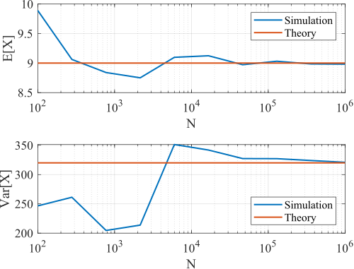
  \(\seteqnumber{0}{2.}{45}\)

  \begin{align*} \lambda &= \frac {1}{2}\\ \E [Y] &= \frac {2}{\left ( \frac {1}{2} \right )^2} + 1 = 9\\ \Var [Y] &= \frac {20}{\left ( \frac {1}{2} \right )^4} = 320 \end{align*}

  

  Figure 2.7: Example of the resulting simulation.

  rng(42)
  N = 1e6;
  x = exprnd(2,[1 N]);
  y = x.^2+1;
  
  
  M = round(logspace(2,6,10));
  for k = 1:length(M)
        E(k) = mean(y(1:M(k)));
        V(k) = var(y(1:M(k)));
  end
  

• (c) The expectation and variance begin to approach the theoretical values as \(N\) increases. However, the numerical result is still not exact even for \(N=10^6\).

Answer of exercise 2.4 

Answer of exercise 2.5 

N = 1e6;         % number of random experiments
X = rand(1,N);   % random experiments
p = nnz(X.^(1/4) < 1/2)/N    % numerical probability

Answer of exercise 3.1 Applying Eq. (3.32f) with the scaling property of the covariance,

\begin{align*} \Var [{\alpha X+\beta Y}] &=\alpha ^2\Var [X] + 2\alpha \beta \Cov [X,Y]+\beta ^2\Var [Y] \end{align*} gives a pair of equations,

\begin{align*} \begin{cases} \Var [X]+4\Cov [X,Y]+4\Var [Y]&=40\\ \Var [X]-4\Cov [X,Y]+4\Var [Y]&=20\\ \Var [X] &= \Var [Y] \end {cases} \end{align*} Adding the first two eliminates the covariance and, with \(\Var [X]=\Var [Y]\), yields \(10\Var [X]=60\). Subtracting them isolates the covariance,

\begin{align*} \Var [X] &= 6=\Var [Y]\\ \Cov [X,Y] &= \frac {20}{8} = 2.5 \end{align*}

Answer of exercise 3.2 Tabulating the joint probabilities,

\[ \begin {array}{ccc} x_k & y_j & p_{XY}[x_k,y_j]\\ \hline -1 & 0 & 1/3\\ -1 & -1 & 1/6\\ 0 & -1 & 1/3\\ 1 & 1 & 1/6 \end {array} \]

the marginals are

\begin{align*} p_X[x] &= \sum _y p_{XY}[x,y] = \begin{cases} \Pr [X=-1] = \tfrac 12,\\ \Pr [X=0] = \tfrac 13,\\ \Pr [X=1] = \tfrac 16, \end {cases}\\ p_Y[y] &= \sum _x p_{XY}[x,y] = \begin{cases} \Pr [Y=-1] = \tfrac 12,\\ \Pr [Y=0] = \tfrac 13,\\ \Pr [Y=1] = \tfrac 16 \end {cases} \end{align*} The two marginals are identical, so \(\E [X]=\E [Y]\) and \(\Var [X]=\Var [Y]\),

\begin{align*} \E [X]= \E [Y] &= (-1)\cdot \frac {1}{2} + 0\cdot \frac {1}{3} + 1\cdot \frac {1}{6} = - \frac {1}{3}\\ \Var [X] = \Var [Y] &= \E [X^{2}] - \bigl (\E [X]\bigr )^2\\ &= \left (1 \cdot \frac {1}{2} + 0\cdot \frac {1}{3} + 1 \cdot \frac {1}{6}\right ) - \left ( - \frac {1}{3} \right )^{2}\\ &= \frac {2}{3} - \frac {1}{9} = \frac {5}{9} \end{align*} The covariance follows from the mixed moment,

\begin{align*} \E [XY] &= \sum _{x,y} x\,y\, p_{XY}[x,y]\\ &= (-1)\cdot 0\cdot \frac {1}{3} + (-1)\cdot (-1)\cdot \frac {1}{6}\\ &\qquad + 0 \cdot (-1) \cdot \frac {1}{3} + 1 \cdot 1 \cdot \frac {1}{6} = \frac {1}{3}\\ \Cov [X,Y] &= \E [XY] - \E [X]\,\E [Y]\\ &= \frac {1}{3} - \left (-\frac {1}{3}\right )\left (-\frac {1}{3}\right ) =\frac {2}{9} \end{align*} and therefore

\[ \rho _{XY} = \frac {\Cov [X,Y]}{\sqrt {\Var [X]\Var [Y]}} = \frac {2/9}{5/9} = \frac {2}{5} \]

Answer of exercise 3.3 The product separates by Eq. (3.24) and the sum by Eqs. (3.22) and (3.34),

\begin{align*} \E [X_i] &= \frac {1}{2},\quad \Var [X_i] = \frac {1}{12}\\ \E [X_i^2] &=\Var [X_i] + \bigl (\E [X_i]\bigr )^2 = \frac {1}{12} + \frac {1}{4} = \frac {1}{3}\\ \E [Y] &= \prod _{i=1}^{n}\E [X_i] = \frac {1}{2^n}\\ \E [Z] &= \sum _{i=1}^{n}\E [X_i] = \frac {n}{2}\\ \Var [Y] &= \E [Y^2] -\bigl (\E [Y]\bigr )^2\\ &=\prod _{i=1}^{n}\E [X_i^2] - \left (\prod _{i=1}^n\E [X_i]\right )^2\\ &=\frac {1}{3^n} -\frac {1}{4^n}\\ \Var [Z] &=\sum _{i=1}^{n}\Var [X_i] =\frac {n}{12} \end{align*}

Answer of exercise 3.4 The exponent is a sum, so the density factors into a function of \(x\) times a function of \(y\),

\begin{multline*} f_{XY}(x,y) = \left [e^{-2x}u(x)\right ]\left [e^{-y/2}u(y)\right ] = f_{X}(x)\,f_{Y}(y) \end{multline*} Each bracket is an exponential density, so condition (3.19a) holds, the variables are independent, and therefore \(\Cov [X,Y]=0\) and \(\rho _{XY}=0\).

Answer of exercise 3.5 

\begin{align*} \E [Y] &= -6\,\E [X] + 22 = -18 + 22 = 4, \\[6pt] \Var [Y] &= \Var [{-6X + 22}] = 36\,\Var [X] = 72, \\[6pt] \E [X^2] &= \Var [X] + \bigl (\E [X]\bigr )^2 = 2 + 9 = 11, \\[6pt] \E [XY] &= \E [{-6X^2 + 22X}] = -6\,\E [X^2] + 22\,\E [X]\\ &= -66 + 66 = 0, \\[6pt] \Cov [X,Y] &= \E [XY] - \E [X]\E [Y] = 0 - 12 = -12, \\[6pt] \rho _{XY} &= \frac {-12}{\sqrt {2\cdot 72}} = -1 \end{align*} Since \(Y\) is an exact linear function of \(X\) with a negative slope, the correlation coefficient attains its lower bound.

Answer of exercise 3.6 The moments of the true radius are

\begin{align*} \E [r] &= \frac {a+b}{2} = 2,\\ \Var [r] &= \frac {(b-a)^2}{12} = \frac {1}{3},\\ \E [r^2] &= \Var [r] + \bigl (\E [r]\bigr )^2 = \frac {13}{3}\approx 4.3333 \end{align*} where \(\E [r^2]\) also follows from Eq. (2.18). The error contributes \(\E [n] = 0\) and \(\E [n^2] = \Var [n] = 0.01\). Because \(r\) and \(n\) are independent,

\begin{align*} \E [X] &= \E [r] + \E [n] = 2,\\ \E [C] &= 2\pi \,\E [X] = 4\pi ,\\[4pt] \Var [X] &= \Var [r] + \Var [n] = \frac {1}{3} + 0.01 \approx 0.3433,\\ \Var [C] &= 4\pi ^2\,\Var [X] \approx 13.5543,\\[4pt] \E [X^2] &= \Var [X] + \bigl (\E [X]\bigr )^2 \approx 4.3433,\\ \E [A] &= \pi \,\E [X^2] \approx 13.6450 \end{align*} The same value of \(\E [X^2]\) is obtained by expanding \(\E [{(r+n)^2}] = \E [r^2] + 2\E [r]\E [n] + \E [n^2]\), in which the middle term vanishes. Finally,

\begin{align*} \E [{Xr}] &= \E [{(r+n)r}] = \E [r^2] + \E [r]\,\cancelto {0}{\E [n]} = \frac {13}{3},\\ \Cov [{X,r}] &= \E [{Xr}] - \E [X]\,\E [r] = \frac {13}{3} - 4 = \frac {1}{3} \end{align*} The covariance equals \(\Var [r]\): the measurement tracks the radius exactly, and the noise adds nothing that the radius shares.

Answer of exercise 3.7 All expectations are taken with the constant density \(f_\Theta (\theta )=1/(2\pi )\) over \([-\pi ,\pi ]\),

\begin{align*} \E [X] &= \frac {1}{2\pi }\int _{-\pi }^{\pi }\cos (\theta )\,d\theta = 0,\\ \E [Y] &= \frac {1}{2\pi }\int _{-\pi }^{\pi }\sin (\theta )\,d\theta = 0,\\ \E [XY] &= \frac {1}{2\pi }\int _{-\pi }^{\pi }\cos (\theta )\sin (\theta )\,d\theta \\ &= \frac {1}{4\pi }\int _{-\pi }^{\pi }\sin (2\theta )\,d\theta = 0,\\ \Cov [X,Y] &= 0 \end{align*} so the pair is uncorrelated. The second moments are

\begin{align*} \E [X^2] &= \frac {1}{2\pi }\int _{-\pi }^{\pi }\cos ^2(\theta )\,d\theta \\ &= \frac {1}{4\pi }\int _{-\pi }^{\pi }\bigl (1+\cos (2\theta )\bigr )\,d\theta = \frac {1}{2} = \E [Y^2] \end{align*} Taking \(g_1(x)=x^2\) and \(g_2(y)=y^2\),

\begin{align*} \E [{X^2Y^2}] &= \frac {1}{2\pi }\int _{-\pi }^{\pi }\cos ^2(\theta )\sin ^2(\theta )\,d\theta = \frac {1}{8} \end{align*} whereas \(\E [X^2]\,\E [Y^2]=\tfrac 14\). The two differ, so Eq. (3.23) fails and the variables are not independent. Indeed \(X^2+Y^2=1\) always, which is as strong a dependence as there is.

Answer of exercise 3.8 Part (a) is Example 3.11 with the sign of \(Y\) reversed, giving Eq. (3.32f). For part (b), substitute \(\Cov [X,Y]=\rho \sigma _1\sigma _2\) from Eq. (3.36),

\begin{align*} \E [{X - Y}] &= \mu _1 - \mu _2,\\ \Var [{X - Y}] &= \sigma _1^2 + \sigma _2^2 - 2\,\rho \,\sigma _1\,\sigma _2 \end{align*}

Answer of exercise 3.9 Each probability is a rectangle, possibly unbounded, so Eq. (3.17) applies. For the first one take \(a = -1\), \(b=1\), \(c=-\infty \), \(d = 1\),

\begin{align*} &\Pr (-1<X<1,\;Y<1)\\ &\quad =F_{XY}(1,1) - F_{XY}(-1,1) - F_{XY}(1,-\infty ) + F_{XY}(-1,-\infty )\\ &\quad =F_{XY}(1,1) - F_{XY}(-1,1) \end{align*} since \(F_X(-\infty )=0\) forces \(F_{XY}(\cdot ,-\infty )=F_{XY}(-\infty ,\cdot )=0\). For the second take \(a = -\infty \), \(b=1\), \(c=-1\), \(d = \infty \),

\begin{align*} &\Pr (X<1,\;-1<Y)\\ &\quad =F_{XY}(1,\infty ) - \cancel {F_{XY}(-\infty ,\infty )} - F_{XY}(1,-1) + \cancel {F_{XY}(-\infty ,-1)}\\ &\quad =F_{X}(1) - F_{XY}(1,-1) \end{align*}

Answer of exercise 3.10 For a jointly Gaussian pair, independence is equivalent to zero covariance by Feature 3.4, so part (a) asks for \(\Cov [V,W]=0\). The two means are

\begin{align*} \E [{V}] &= \E [{X_1}]\cos (\theta )+\E [{X_2}]\sin (\theta ) = m\left [\cos (\theta ) + \sin (\theta )\right ]\\ \E [{W}] &= -\E [{X_1}]\sin (\theta )+\E [{X_2}]\cos (\theta ) = m\left [\cos (\theta ) - \sin (\theta )\right ]\\ \E [{V}]\E [{W}] &= m^2\left [\cos ^2(\theta ) - \sin ^2(\theta )\right ] = m^2\cos (2\theta ) \end{align*} For the mixed moment, the two terms carrying \(\E [X_1^2]\) and \(\E [X_2^2]\) cancel because the two variances are equal, and the remaining terms combine into \(\cos (2\theta )\),

\begin{align*} \E [{VW}] &= -\E [{X_1^2}]\sin (\theta )\cos (\theta )+\E [{X_2^2}]\sin (\theta )\cos (\theta )\\ &\qquad + \E [{X_1X_2}]\bigl (\cos ^2(\theta ) - \sin ^2(\theta )\bigr )\\ & = \E [{X_1X_2}]\cos (2\theta ) \end{align*} so that

\begin{align*} \Cov [V,W] &= \bigl (b - m^2\bigr )\cos (2\theta ) \end{align*} With \(b\ne m^2\) this vanishes when \(\cos (2\theta )=0\), that is

\[ \theta = \frac {\pi }{2}n - \frac {\pi }{4},\quad n\in \mathbb {Z}, \]

which inside \([-\pi ,\pi ]\) means \(\theta \in \left \lbrace -\tfrac {3\pi }{4},-\tfrac {\pi }{4},\tfrac {\pi }{4},\tfrac {3\pi }{4}\right \rbrace \).

For part (b), \(V\) and \(W\) are linear combinations of a jointly Gaussian pair, so by Definition 3.4 they are themselves jointly Gaussian. Their distribution is therefore Eq. (3.41) with the five parameters

\begin{align*} \E [V] &= m\bigl (\cos \theta + \sin \theta \bigr ),\\ \E [W] &= m\bigl (\cos \theta - \sin \theta \bigr ),\\ \Var [V] &= \E [V^2] - \bigl (\E [V]\bigr )^2,\\ \Var [W] &= \E [W^2] - \bigl (\E [W]\bigr )^2,\\ \rho _{VW} &= \frac {(b-m^2)\cos (2\theta )}{\sqrt {\Var [V]\Var [W]}} \end{align*} where \(\E [V^2]\) and \(\E [W^2]\) are expanded from the definitions of \(V\) and \(W\) in the same way as \(\E [{VW}]\) above.

Answer of exercise 3.11 The sum equals one when exactly one of the three variables is one. The three cases are disjoint, and each is a product of three independent probabilities,

\begin{align*} \Pr (X_1+X_2+X_3 = 1) &=\Pr [X_1=1]\Pr [X_2=0]\Pr [X_3=0] \\ &\quad + \Pr [X_1=0]\Pr [X_2=1]\Pr [X_3=0]\\ &\quad + \Pr [X_1=0]\Pr [X_2=0]\Pr [X_3=1]\\ &=p_1(1-p_2)(1-p_3) + (1-p_1)p_2(1-p_3)\\ &\quad + (1-p_1)(1-p_2)p_3 \end{align*} The sum equals two when exactly one of them is zero,

\begin{align*} \Pr (X_1+X_2+X_3 = 2) &=p_1p_2(1-p_3) + p_1(1-p_2)p_3\\ &\quad + (1-p_1)p_2p_3 \end{align*} A simulation draws three Bernoulli sequences and counts the sums,

N   = 1e6;
p   = [0.2 0.4 0.7];
X   = rand(3,N) < p(:);
S   = sum(X,1);
p1 = nnz(S == 1)/N
p2 = nnz(S == 2)/N

Answer of exercise 3.12 

N = 1e6;         % number of random experiments
X = rand(1,N);   % random experiments
Y = rand(1,N);   %
p = nnz(X.^(1/3) > Y/2)/N    % numerical probability

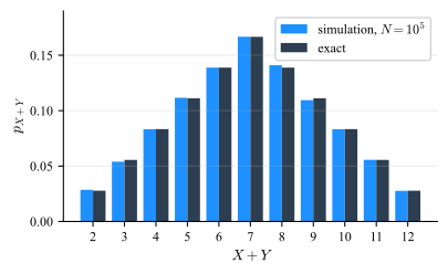
Answer of exercise 3.13 Draw two independent sequences of faces, add them, count how many times each sum occurs and divide by the number of trials. The result is shown in the figure below.

N = 1e5;
X = randi(6,1,N);
Y = randi(6,1,N);
S = X + Y;
p = histcounts(S, 1.5:1:12.5)/N

Answer of exercise 4.1 With a single coefficient the derivation needs only one derivative,

\begin{align*} \MSE (a) &= \E [{(Y-aX)^2}] = \E [Y^2] - 2a\E [XY] + a^2\E [X^2]\\ \frac {d}{da}\MSE (a) &= - 2\E [XY] + 2a\E [X^2] = 0\\ a_{opt} &=\frac {\E [XY]}{\E [X^2]} \end{align*} Note that the moments are not centered here, because the predictor has no offset to absorb the means. Consequently the mean error does not vanish,

\begin{align*} \E [{Y - \hat {Y}}] &= \E [Y] - \frac {\E [XY]}{\E [X^2]}\E [X]\\ \MSE _{min} &=\E [Y^2] - \frac {\bigl (\E [XY]\bigr )^2}{\E [X^2]} \end{align*} which should be contrasted with Feature 4.2.

Answer of exercise 4.2 The derivation is the same as for the constant and linear cases, with \(X^2\) in place of \(X\),

\begin{align*} \MSE (a) &=\E [{(Y-aX^2)^2}]\\ &=\E [Y^2]-2a\,\E [{X^2Y}] + a^2\E [X^4]\\ \frac {\partial }{\partial a}\MSE (a) &= -2\E [{X^2Y}] + 2a\E [X^4] = 0\\ a_{opt} &= \frac {\E [{X^2Y}]}{\E [X^4]}\\ \MSE _{min} &=\E [Y^2] - \frac {\bigl (\E [{X^2Y}]\bigr )^2}{\E [X^4]} \end{align*} Every moment needed below follows from the uniform moments

\[ \E [W_i^n]=\int _{0}^{1}x^n\,dx = \frac {1}{n+1},\qquad i=1,2 \]

and from the independence of \(W_1\) and \(W_2\),

\begin{align*} \E [Y^2] &=\E [W_1^4] = \frac {1}{5} = 0.2\\ \E [{X^2Y}] &=\E [{\left (\tfrac {9}{10}W_1 + \tfrac {1}{10}W_2\right )^2W_1^2}]\\ &= \left (\frac {9}{10}\right )^2 \E [W_1^4] + 2\cdot \frac {9}{10}\cdot \frac {1}{10}\E [W_1^3]\E [W_2]\\ &\qquad + \left (\frac {1}{10}\right )^2 \E [W_1^2]\E [W_2^2] \\ &= \left (\frac {9}{10}\right )^2 \frac {1}{5} + \frac {18}{100}\cdot \frac {1}{4}\cdot \frac {1}{2} + \frac {1}{100}\cdot \frac {1}{3}\cdot \frac {1}{3}\\ &=\frac {3341}{18\,000}\approx 0.18561 \\ \E [X^4] &=\E [{\left (\tfrac {9}{10}W_1 +\tfrac {1}{10}W_2\right )^4}]\\ &=\left (\frac {9}{10}\right )^4\frac {1}{5} + 4\left (\frac {9}{10}\right )^3\frac {1}{10}\cdot \frac {1}{4}\cdot \frac {1}{2}\\ &\qquad + 6\left (\frac {9}{10}\right )^2\left (\frac {1}{10}\right )^2\frac {1}{3}\cdot \frac {1}{3}\\ &\qquad + 4\cdot \frac {9}{10}\left (\frac {1}{10}\right )^3\frac {1}{2}\cdot \frac {1}{4} +\left (\frac {1}{10}\right )^4\frac {1}{5}\\ &=\frac {8\,677}{50\,000}\approx 0.17354\\ \MSE _{min} &=\frac {83\,111}{56\,226\,960}\approx 1.478\times 10^{-3} \end{align*} For the linear predictor, the same moments give

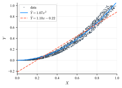
\begin{align*} \Var [X] &=\left (\frac {9}{10}\right )^2\frac {1}{12} + \left (\frac {1}{10}\right )^2\frac {1}{12} =\frac {41}{600}\approx 0.06833\\ \Var [Y] &=\E [W_1^4] - \bigl (\E [W_1^2]\bigr )^2 =\frac {1}{5} - \frac {1}{9}=\frac {4}{45}\approx 0.08889\\ \Cov [X,Y] &=\frac {9}{10}\E [W_1^3] + \frac {1}{10}\E [W_1^2]\E [W_2]\\ &\qquad - \E [W_1^2]\left (\frac {9}{10}\E [W_1]+ \frac {1}{10}\E [W_2]\right ) =\frac {3}{40}\\ \MSE _{min} &=\Var [Y]\left (1-\rho _{XY}^2\right ) =\frac {97}{14\,760}\approx 6.572\times 10^{-3} \end{align*} The quadratic predictor is roughly four times more accurate. This is expected: \(Y\) is a squared function of \(W_1\), and \(X\) is almost \(W_1\), so the true relation between \(X\) and \(Y\) is close to quadratic, as the figure below shows. A straight line can only approximate it, and Eq. (4.15) measures exactly that shortfall.

Answer of exercise 4.3 Writing the data as a joint PDF table,

\[ \begin {array}{ccc} x_k & y_j & p_{XY}[x_k,y_j]\\ \hline 0 & 0 & 1/4\\ 1 & 1 & 1/4\\ 2 & 2 & 1/4\\ 2 & 3 & 1/4 \end {array} \]

the value \(x=2\) occurs twice, so its marginal probability is doubled,

\[ p_X[x] = \begin {cases} 1/4 & x = 0\\ 1/4 & x = 1\\ 1/2 & x = 2 \end {cases} \qquad p_Y[y] = \begin {cases} 1/4 & y = 0\\ 1/4 & y = 1\\ 1/4 & y = 2\\ 1/4 & y = 3 \end {cases} \]

\begin{align*} \E [X] &= \frac {1}{4}\cdot 0 + \frac {1}{4}\cdot 1 + \frac {1}{2}\cdot 2 = \frac {5}{4}\\ \E [Y] &= \frac {1}{4}\left (0 + 1 + 2 + 3\right ) = \frac {3}{2}\\ \E [X^2] &= \frac {1}{4}\cdot 1 + \frac {1}{2}\cdot 4 = \frac {9}{4}\\ \E [Y^2] &= \frac {1}{4}\left (0 + 1 + 4 + 9\right ) = \frac {14}{4}\\ \Var [X] &= \E [X^2] - \bigl (\E [X]\bigr )^2 = \frac {9}{4}-\frac {25}{16} = \frac {11}{16} \\ \Var [Y] &= \E [Y^2] - \bigl (\E [Y]\bigr )^2 = \frac {14}{4} - \frac {9}{4} = \frac {5}{4} \\ \E [XY] &= \frac {1}{4}\left (0\cdot 0 + 1\cdot 1 + 2\cdot 2 + 2\cdot 3\right ) = \frac {11}{4} \\ \Cov [X,Y] &= \E [XY] - \E [X]\E [Y] = \frac {11}{4} - \frac {15}{8} = \frac {7}{8} \\ \rho _{XY} &=\frac {7/8}{\sqrt {\frac {11}{16}\cdot \frac {5}{4}}} \approx 0.944\\ \hat {Y} &=\E [Y]+\frac {\Cov [X,Y]}{\Var [X]}\bigl (x-\E [X]\bigr ) = \frac {14}{11}x-\frac {1}{11} \end{align*}

Answer of exercise 4.4 The values of \(X\) are symmetric about zero, so \(\E [X]=0\) and the covariance reduces to the mixed moment,

\begin{align*} \E [X] &= 0\\ \Var [X] &= \frac {1}{5}\left (4+1+0+1+4\right ) =2\\ \E [Y] &= \frac {1}{5}\left (0+0+3+3+4\right ) = 2\\ \Var [Y] &=\frac {1}{5}\left (4 + 4 + 1 + 1 + 4\right ) = \frac {14}{5} = 2.8\\ \E [XY]&= \frac {1}{5}\left (0+0+0+3+8\right ) = \frac {11}{5} = 2.2\\ \Cov [X,Y] &= \E [XY] - \E [X]\E [Y] = \frac {11}{5} \end{align*} Substituting into Eqs. (4.14) and (4.15),

\begin{align*} \hat {Y} &= 2 + \frac {11}{5}\cdot \frac {1}{2}\,x = 2+ \frac {11}{10}\cdot 1 = 3.1\\ \rho _{XY} &= \frac {11/5}{\sqrt {2.8\cdot 2}}\approx 0.9297\\ \MSE _{min} &= \Var [Y]\bigl (1-\rho _{XY}^2\bigr )\approx 0.38 \end{align*} The same computation in code:

X = [-2 -1 0 1 2];
Y = [0 0 3 3 4];
Ex = mean(X); Ey = mean(Y);
VarX = mean((X-Ex).^2); VarY = mean((Y-Ey).^2);
CovXY = mean(X.*Y) - Ex*Ey;
rho = CovXY/sqrt(VarX*VarY)
VarY*(1 - rho^2)

Answer of exercise 4.5 Summing the rows and the columns of the table gives the marginals,

\begin{align*} p_X[x] &= \left \lbrace 0.2,\; 0.3,\; 0.3,\; 0.2\right \rbrace , \quad x=1,\ldots ,4\\ p_Y[y] &= \left \lbrace 0.3,\; 0.4,\; 0.3\right \rbrace , \quad y=1,2,3 \end{align*} from which

\begin{align*} \E [X] &= 1\cdot 0.2 + 2\cdot 0.3 + 3\cdot 0.3 + 4\cdot 0.2=2.5\\ \E [X^2] &= 1\cdot 0.2 + 4\cdot 0.3 + 9\cdot 0.3 + 16\cdot 0.2=7.3\\ \Var [X] &=\E [X^2]-\bigl (\E [X]\bigr )^2 = 1.05\\ \E [Y] &= 1\cdot 0.3 + 2\cdot 0.4 + 3\cdot 0.3=2\\ \E [Y^2] &= 1\cdot 0.3 + 4\cdot 0.4 + 9\cdot 0.3=4.6\\ \Var [Y] &=\E [Y^2] - \bigl (\E [Y]\bigr )^2 = 0.6 \end{align*} The mixed moment runs over the six non-zero cells only,

\begin{align*} \E [XY] & = 1\cdot 3\cdot 0.2 + 2\cdot 2\cdot 0.2 + 2\cdot 3\cdot 0.1\\ &\quad + 3\cdot 1\cdot 0.1 + 3\cdot 2\cdot 0.2 + 4\cdot 1\cdot 0.2 = 4.3\\ \Cov [X,Y] &=\E [XY] - \E [X]\E [Y] = 4.3 - 5 = -0.7\\ \rho _{XY} &= \frac {-0.7}{\sqrt {1.05\cdot 0.6}} = -\frac {\sqrt {7}}{3} \approx -0.882\\ \hat {y} &= \E [Y] + \frac {\Cov [X,Y]}{\Var [X]}\bigl (x-\E [X]\bigr )\\ &= 2 - \frac {0.7}{1.05}\left (3-2.5\right ) \approx 1.667 \end{align*} The correlation is strongly negative, and the predicted \(y\) at \(x=3\) accordingly falls below \(\E [Y]\).

Answer of exercise 4.6 The marginals are row and column sums of the joint PDF,

\begin{align*} p_{X}[1] &= p_{XY}[1,0] + p_{XY}[1,1] = p_1 = 0.6\\ p_Y[1] &=p_{XY}[0,1] + p_{XY}[1,1] = p_2 = 0.8 \end{align*} By Eqs. (4.6) and (4.7) the best constant is the expectation and its error is the variance,

\begin{align*} b_x &=\E [X] = p_1 = 0.6\\ \MSE _{min} &=\Var [X] = p_1(1-p_1) = 0.24 \end{align*} The same two results applied to \(Z\), using the linearity of the expectation and Eq. (3.34) for the variance of a sum of independent variables,

\begin{align*} b_z &=\E [Z] = a\E [X] + c\E [Y]= ap_1 + cp_2\\ \MSE _{min} &=\Var [Z] = a^2 p_1(1-p_1) + c^2 p_2(1-p_2)\\ &= 0.24a^2 + 0.16c^2 \end{align*} For the last part, expand the covariance of \(X\) with \(Z\). The term in \(\E [XY]\) factors because \(X\) and \(Y\) are independent, and it cancels exactly,

\begin{align*} \E [XZ] &=a\E [X^2] + c\,\E [X]\E [Y] = ap_1 + cp_1p_2\\ \Cov [X,Z] &=\E [XZ]-\E [X]\E [Z]\\ &=ap_1 + cp_1p_2 - p_1\left (ap_1+cp_2\right )\\ &=a\left (p_1-p_1^2\right ) = a\Var [X] \end{align*} where \(\E [X^2]=p_1\) because \(X\) takes only the values \(0\) and \(1\). Since \(\Var [X]>0\) for \(0<p_1<1\), the covariance vanishes only for \(a=0\). No such pair of non-zero constants exists: the contribution of \(Y\) to \(Z\) is irrelevant here, and only removing \(X\) from \(Z\) can decorrelate them.

Answer of exercise 4.7 From the definition of the correlation coefficient, Eq. (3.36), with \(\sigma _X=2\) and \(\sigma _Y=1\),

\[ \Cov [X,Y] = \rho _{XY}\sigma _X\sigma _Y = \frac {1}{2}\cdot 2 \cdot 1 = 1 \]

Both means are zero, so the second moment of the sum is its variance,

\[ \begin {aligned} \E [{(X+Y)^2}] &= \Var [{X+Y}]\\ &=\Var [X]+\Var [Y]+2\Cov [X,Y]\\ &=4+1+2 = 7 \end {aligned} \]

Because the means are zero, the offset of Eq. (4.13b) vanishes and the predictor reduces to the single coefficient of Eq. (4.13a), with the roles of \(X\) and \(Y\) exchanged,

\[ a = \frac {\Cov [X,Y]}{\Var [Y]} = 1 \quad \Longrightarrow \quad \hat X = Y \]

The error follows either directly or from Eq. (4.15),

\[ \begin {aligned} \E [{(X-Y)^2}] &= \Var [{X-Y}] = \Var [X] + \Var [Y] - 2\Cov [X,Y]\\ &= 4 + 1 - 2 = 3\\ &= \Var [X]\bigl (1-\rho _{XY}^2\bigr ) = 4\left (1-\frac {1}{4}\right ) = 3 \end {aligned} \]

Finally, \(X+Y\) is a linear combination of a jointly Gaussian pair, hence Gaussian, with zero mean and variance \(7\),

\[ \Pr (X+Y>1) = Q\left (\frac {1}{\sqrt {7}}\right ) \approx 0.354 \]

Answer of exercise 4.8 The covariance of the first pair follows from Eq. (3.36),

\[ \Cov [X_1,X_2] = \rho _{X_1X_2}\,\sigma _1\sigma _2 = \frac {1}{\sqrt 2}\cdot 1\cdot \sqrt 2 = 1 \]

so that, by Eq. (4.14),

\[ \hat X_2 = \E [X_2] + \frac {\Cov [X_1,X_2]}{\Var [X_1]}\,\bigl (x_1-\E [X_1]\bigr ) = 1 + x_1 \]

For the second pair, expanding each quantity with Eqs. (3.22) and (3.32f),

\[ \E [Y_3]=2,\quad \E [Y_4]=2,\quad \Var [Y_3]=13,\quad \Var [Y_4]=29,\quad \Cov [Y_3,Y_4]=19 \]

gives

\[ \hat Y_4 = \E [Y_4] + \frac {\Cov [Y_3,Y_4]}{\Var [Y_3]}\,\bigl (y_3-\E [Y_3]\bigr ) =2 + \frac {19}{13}\,(y_3-2) \]

with \(\rho _{Y_3Y_4} = 19/\sqrt {13\cdot 29}\approx 0.979\).

For the last part, compare the stated variances with what Eq. (3.32f) predicts. If the two variables were independent the cross term would vanish, and the variance would come out smaller,

\[ \Var [Y_2] =\Var [X_1] + 4\Var [X_3] - 4\,\Cov [X_1,X_3] = 3 \;\Longrightarrow \;\Cov [X_1,X_3] = \tfrac 12 \ne 0, \]

\[ \Var [Y_1] =\Var [X_2] + \Var [X_3] + 2\,\Cov [X_2,X_3] = 5 \;\Longrightarrow \;\Cov [X_2,X_3] = 1 \ne 0 \]

A non-zero covariance rules out independence, by Feature 3.3.1, so neither pair is independent.

Finally, every linear combination of \(Y_3\) and \(Y_4\) is a linear combination of the jointly Gaussian \(X_1\) and \(X_2\), hence Gaussian. By Definition 3.4, \(Y_3\) and \(Y_4\) are jointly Gaussian. Their joint distribution is the bivariate Gaussian PDF (3.41), with the five numbers already computed:

\[ \mu _{Y_3}=\mu _{Y_4}=2,\qquad \sigma _{Y_3}^2=13,\qquad \sigma _{Y_4}^2=29,\qquad \rho _{Y_3Y_4}\approx 0.979 . \]

Answer of exercise 4.9 The perimeter and the area are

\[ C = 2X + 2Y, \qquad A = X\,Y \]

Using \(\E [X]=\tfrac 12\), \(\E [X^2]=\tfrac 13\) and the independence of \(X\) and \(Y\),

\begin{align*} \E [C]&=2\bigl (\E [X]+\E [Y]\bigr )=2, & \E [A]&=\E [X]\E [Y]=\tfrac 14,\\ \end{align*}

\begin{align*} \E [{CA}]&=2\bigl (\E [X^2]\E [Y]+\E [X]\E [Y^2]\bigr ) =\tfrac 23,\\ \Cov [C,A]&=\E [{CA}]-\E [C]\E [A] =\tfrac 23 - \tfrac 12 =\tfrac 16 \end{align*} Here \(A\) is the observed variable, so it takes the place of \(X\) in Eq. (4.14),

\[ \hat C =\E [C] + \frac {\Cov [C,A]}{\Var [A]}\bigl (A - \E [A]\bigr ) \]

with

\[ \Var [A] =\E [X^2]\E [Y^2]-\bigl (\E [X]\E [Y]\bigr )^2 =\tfrac {1}{9}-\tfrac {1}{16} =\tfrac {7}{144}, \]

so that

\[ \hat C =2 + \frac {1/6}{7/144}\left (A-\tfrac 14\right ) =\frac {24}{7}\,A + \frac {8}{7} \]

For the error, the variance of the perimeter and the correlation coefficient are

\begin{align*} \Var [C] &=4\Var [X]+4\Var [Y] =\tfrac 23,\\ \rho _{CA} &=\frac {\Cov [C,A]}{\sqrt {\Var [C]\,\Var [A]}} =\frac {\sqrt {42}}{7} \end{align*} and therefore

\[ \MSE _{min} = \Var [C] \bigl (1 - \rho _{CA}^{2}\bigr ) = \frac {2}{3} \left ( 1 - \frac {42}{49} \right ) = \frac {2}{21} \approx 0.0952 \]

Answer of exercise 5.1 

• (a)

  \(\seteqnumber{0}{5.}{24}\)

  \begin{align*} \bar {x} &= \frac {1}{8}\left (2+4+4+4+5+5+7+9\right ) = \frac {40}{8} = 5\\ x_i-\bar {x} &= -3,\ -1,\ -1,\ -1,\ 0,\ 0,\ 2,\ 4\\ \sum _i\left (x_i-\bar {x}\right )^2 &= 9+1+1+1+0+0+4+16 = 32 \end{align*} The deviations sum to zero, which is the arithmetic check on \(\bar {x}\).

• (b)

  \(\seteqnumber{0}{5.}{24}\)

  \begin{align*} s^2_{\text {biased}} &= \frac {32}{n} = \frac {32}{8} = 4, & s_{\text {biased}} &= 2\\ s^2_{\text {unbiased}} &= \frac {32}{n-1} = \frac {32}{7} \approx 4.571, & s_{\text {unbiased}} &\approx 2.138 \end{align*}

• (c) The data are already sorted. With \(n=8\) even, the median is the average of the two central order statistics, \(x_{(4)}=4\) and \(x_{(5)}=5\),

  \(\seteqnumber{0}{5.}{24}\)

  \begin{equation*} \text {median} = \frac {4+5}{2} = 4.5,\qquad \text {mode} = 4 \ \ (\text {three occurrences}),\qquad \text {range} = 9-2 = 7 . \end{equation*}

• (d) The two estimators differ by a fixed factor that depends on \(n\) alone,

  \(\seteqnumber{0}{5.}{24}\)

  \begin{equation*} \frac {s^2_{\text {biased}}}{s^2_{\text {unbiased}}} = \frac {n-1}{n}, \qquad \text {here}\qquad \frac {7}{8} = 0.875 , \end{equation*}

  a \(12.5\%\) gap, far too large to ignore. The relative gap is \(1/n\), the relative bias of Example 5.2, so the choice stops mattering at \(n\ge 100\).

• (e) The standard error (5.16) takes the unbiased \(s\) of part (b), since that is the normalization the \(t\) quantiles are tabulated for,

  \(\seteqnumber{0}{5.}{24}\)

  \begin{align*} \widehat {\mathrm {SE}}(\bar {x}) &= \frac {s_{\text {unbiased}}}{\sqrt {n}} = \frac {2.138}{\sqrt {8}} = 0.756\\ t_{7,\,0.975}\cdot \widehat {\mathrm {SE}}(\bar {x}) &= 2.365\cdot 0.756 = 1.788\\ \bar {x} \pm 1.788 &= \left [3.21,\ 6.79\right ] \end{align*} by (5.18), with \(n-1=7\) degrees of freedom.

  The interval is \(3.58\) wide against a range of \(7\): the uncertainty about where the center sits covers half the spread of the data itself. Eight readings place this sensor at \(5\pm 1.8\), and the choice between the two variance normalizations, worth \(12.5\%\) in part (d), cannot compete with that. Deciding how many samples to take is the first-order question; deciding how to normalize them is a detail.

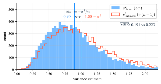
Answer of exercise 5.2 With \(\sigma ^2=1\) and \(n=10\) the four targets are

\begin{align*} \E [s^2_{\text {unbiased}}] &= 1, &\overline {\mathrm {MSE}}_{\text {unbiased}} &= \frac {2}{9} \approx 0.2222\\ \E [s^2_{\text {biased}}] &= \frac {9}{10} = 0.9, &\overline {\mathrm {MSE}}_{\text {biased}} &= \frac {19}{100} = 0.19 \end{align*} At \(k=10^4\) the simulated means should land within about \(1\%\) of these, by (5.22); the simulated MSEs are themselves averages and settle a little more slowly.

• (a) The unbiased estimator averages to \(1\) and the biased one to \(0.9\), the \(10\%\) shortfall predicted by the bias \(-\sigma ^2/n\).

• (b) The biased estimator has the smaller MSE, \(0.19\) against \(0.2222\), about \(14\%\) lower. Dividing by \(n\) rather than \(n-1\) shrinks every estimate slightly, and shrinking a noisy positive quantity costs a little bias but removes more variance than that. Unbiasedness and accuracy are two different goals, and here they point in opposite directions.

• (c) For a single number reported once, the biased estimator is the better bet, and it is the book’s default. The unbiased one earns its place where the bias would accumulate, most importantly inside the confidence bounds of Sec. 5.2.2, whose \(t\) and \(\chi ^2\) quantiles are tabulated for the \(n-1\) normalization. Both effects vanish as \(n\) grows: at \(n=100\) the gap in either column is around \(1\%\).

Answer of exercise 6.1 

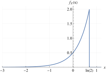
\begin{align*} \int _{-\infty }^{\infty }f_X(x)\,dx &= 1\\ \Rightarrow \int _{-\infty }^{\ln (a)}\frac {1}{2}e^{2x}\,dx&=\frac {1}{4}e^{2x}\Big |_{-\infty }^{\ln (a)}=\frac {1}{4}a^2=1 \Rightarrow \abs {a}=2 \end{align*} Note: \(a\) cannot be negative, because of \(\ln (a)\).

\begin{align*} F_X(x)&=\int ^{x}_{-\infty }f_X(x)\,dx= \int ^{x}_{-\infty }\frac {1}{2}e^{2x}\,dx = \begin{cases} \frac {1}{4}e^{2x} & x<\ln (2) \\ 1 & x>\ln (2) \end {cases}\\ \E [X] &=\int ^{\ln (2)}_{-\infty }x\cdot \frac {1}{2}e^{2x}\,dx\\ &=\frac {1}{8}e^{2x}\left [2x-1\right ]\Big |_{-\infty }^{\ln (2)}\\ &=\frac {1}{8}\bigl (e^{2\ln (2)}=4\bigr )\left [2\ln (2)-1\right ]\\ &={\ln \left (2\right )\ }-\frac {1}{2}\approx 0.193147 \end{align*}

\begin{align*} \E [X^2] &=\frac {1}{2}\int _{-\infty }^{\ln (2)}x^2e^{2x}\,dx\\ &=\frac {1}{2}\cdot e^{2x}\left [\frac {x^2}{2} - \frac {2x}{2^2} + \frac {2}{2^3}\right ]\bigg |_{-\infty }^{\ln (2)}\\ &= \frac {1}{2}\cdot 4 \left [\frac {\ln ^2(2)}{2} - \frac {\ln (2)}{2} + \frac {1}{4} \right ]\\ &= \ln ^2(2) - \ln (2) + \frac {1}{2}\approx 0.287306\\ \Var [X] &= \E [X^2] - \bigl (\E [X]\bigr )^2 = \frac {1}{4} \\ \Pr (X<0) &=\int _{-\infty }^{0}f_X(x)\,dx = \int _{-\infty }^{0}\frac {1}{2}e^{2x}\,dx\\ &= \frac {1}{2}\cdot \frac {1}{2} e^{2x}\Big |_{-\infty }^{0}=\frac {1}{4}\left (1 - 0\right ) = \frac {1}{4}\\ F_X(x_0) &= \frac {1}{2} = \frac {1}{4}e^{2x_0} \quad \Rightarrow e^{2x_0} = 2 \quad \Rightarrow 2x_0 = \ln (2)\\ x_0 &= \frac {\ln (2)}{2}\approx 0.34657359 \end{align*} For the histogram, since \(X<\ln (2)<1\) the interval \((0,1)\) captures all positive values,

\begin{align*} \Pr (0<X<1) &= 1- \Pr (X<0) = \frac {3}{4} \\ &= \int _{0}^{\ln (2)}\frac {1}{2}e^{2x}\,dx =\frac {1}{4}\left (2^2 - 1\right )=\frac {3}{4}\\ n &= N\cdot \Pr (0<X<1) = 100{,}000\cdot \frac {3}{4} = 75{,}000\\ \hat {f}_X(0.5) &= \frac {n}{N} \frac {1}{\Delta x} = \Pr (0<X<1)\frac {1}{\Delta x} = \frac {3}{4}\cdot \frac {1}{1} = \frac {3}{4} \end{align*}

Answer of exercise 6.2 Given: \(N=500\), \(\Delta x = 4\), \(n_i = 80\).

• (a)

  • (1) count: the height is the number of outcomes in the bin, \(H_{\mathrm {count}} = n_i = 80\).

  • (2) probability: the height is the relative frequency,

    \[ H_{\mathrm {prob}} = \frac {n_i}{N} = \frac {80}{500} = 0.16 . \]

  • (3) pdf: the relative frequency is normalized by the bin width,

    \[ H_{\mathrm {pdf}} \approx f_X(x_i) = \frac {n_i}{N \cdot \Delta x} = \frac {80}{500 \cdot 4} = \frac {80}{2000} = 0.04 . \]

• (b) In a pdf histogram the probability is represented by the area. The area of the rectangle is

  \[ H_{\mathrm {pdf}} \cdot \Delta x = 0.04 \cdot 4 = 0.16 = H_{\mathrm {prob}} . \]

  It is the estimated probability that \(X\) falls within the bin \([10, 14]\), and it equals the height of the probability type, as expected.

• (c) From the pdf histogram formula,

  \[ H_{\mathrm {pdf}} = \frac {n_j}{N \cdot \Delta x} \;\Longrightarrow \; 0.03 = \frac {n_j}{500 \cdot 4} = \frac {n_j}{2000} \;\Longrightarrow \; n_j = 0.03 \cdot 2000 = 60 . \]

  Sixty outcomes were counted in the bin \([20, 24]\).

Answer of exercise 6.3 

• (a) The draw spans about \([-3.9,\,3.1]\), so the bin width is roughly \(7/k\) and a central bin holds close to \(N\,f_X(0)\,\Delta x \approx 1000\cdot 0.4\cdot 7/k \approx 2800/k\). The counts therefore fall as \(1/k\): every halving of the bin width halves the evidence behind each bar. One run gives

  .
  \(k\)	\(\Delta x\)	central \(n_i\)	\(1/\sqrt {n_i}\)	bins below \(25\) counts
  5	1.39	496	\(4.5\%\)	1 of 5
  20	0.35	128	\(8.8\%\)	9 of 20
  100	0.07	34	\(17.1\%\)	86 of 100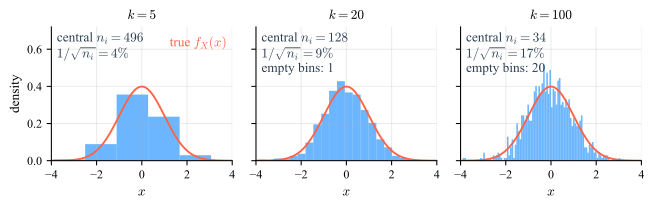

  

  Figure 6.11: The same \(N=1000\) draw at three bin widths, with the true density overlaid, so every difference between the panels comes from \(\Delta x\) alone. At \(k=5\) the bars are steady but the bell is gone; at \(k=100\) the shape is right on average and the individual bars are not, with \(20\) bins empty; \(k=20\) balances the two.

• (b) At \(k=20\): the bins are narrow enough to resolve the peak and wide enough that each bar is reliable to about \(9\%\). The other two fail for opposite reasons. At \(k=5\) the bars are steady, and visibly wrong: five bars cannot render a bell, and each one averages the density over a full standard deviation, so the peak is flattened and the tails are overstated; the error is not noise but bin width. At \(k=100\) the bars follow the curve on average but scatter around it by roughly a fifth of their height, and the tail bins, holding a handful of samples each, suggest structure that is not there.

• (c) The central bin clears \(25\) counts in all three cases, so judging a histogram by its peak is no test at all. The last column of the table is the one that matters: at \(k=20\) nearly half the bins already fall below the rule, and at \(k=100\) so do \(86\) of them, with \(20\) holding nothing whatsoever. The tails always run out of samples first, and \(N\) and \(k\) have to grow together, since the relative error depends on \(n_i \approx N/k\) alone.

Answer of exercise 7.1 Panels (a), (b) and (d) are all straight, so they are ordered by how tightly the points hug the line; panel (c) is both curved and the most scattered, so it comes last. The ranking is (b), (a), (d), (c), with

\[ r_{xy} = \begin {cases} -0.991 & \text {(a)},\\ +0.997 & \text {(b)},\\ +0.835 & \text {(c)},\\ -0.941 & \text {(d)} \end {cases} \]

The sign plays no part in the ranking: panel (a) has a negative slope and still outranks panel (d), whose slope is also negative but whose scatter is larger.

Answer of exercise 7.2 

• (a) Clean data. With \(\bar {x} = 3.5\) and \(\bar {y} = 63/6 = 10.5\),

  .
  \(k\)	1	2	3	4	5	6	\(\sum \)
  \(x_k-\bar {x}\)	\(-2.5\)	\(-1.5\)	\(-0.5\)	0.5	1.5	2.5	0
  \(y_k-\bar {y}\)	\(-9.5\)	\(-8.5\)	\(-6.5\)	\(-2.5\)	5.5	21.5	0
  product	23.75	12.75	3.25	\(-1.25\)	8.25	53.75	100.5

  \(\seteqnumber{0}{7.}{44}\)

  \begin{equation*} r_{xy} = \frac {100.5}{\sqrt {17.5\cdot 703.5}} = \frac {100.5}{110.96} \approx 0.906 . \end{equation*}

  Noisy data. Swapping \(y_3\) and \(y_4\) leaves \(\bar {y}\) and \(\sum (y_k-\bar {y})^2\) untouched, so only the cross term changes,

  \(\seteqnumber{0}{7.}{44}\)

  \begin{equation*} \sum _k\left (x_k-\bar {x}\right )\left (y_k-\bar {y}\right ) = 23.75+12.75+1.25-3.25+8.25+53.75 = 96.5, \qquad r_{xy} = \frac {96.5}{110.96} \approx 0.870 . \end{equation*}

• (b) Clean data. Both \(x\) and \(y\) increase strictly, so both rank vectors are \(1,2,3,4,5,6\) and they are identical, \(r_s = r_{R(x)R(y)} = 1\).

  Noisy data. The ranks of \(y\) become \(1,2,4,3,5,6\). With \(R(x)\) still \(1,\dots ,6\) and both rank vectors having the same spread \(\sum (R-\bar {R})^2 = 17.5\),

  \(\seteqnumber{0}{7.}{44}\)

  \begin{equation*} \sum _k\left (R(x_k)-\bar {R}\right )\left (R(y_k)-\bar {R}\right ) = 6.25+2.25-0.25-0.25+2.25+6.25 = 16.5, \qquad r_s = \frac {16.5}{17.5} \approx 0.943 . \end{equation*}

• (c) In the clean case the relation is perfect but not linear, and the two coefficients say exactly that: \(r_s=1\) certifies the perfect monotonicity, while \(r_{xy}=0.906\) reports only how well a straight line approximates a doubling curve. The shortfall in \(r_{xy}\) is a statement about the model, not about the data.

  In the noisy case a single pair is out of order. \(r_s\) drops to \(0.943\), and it drops for the right reason: monotonicity is genuinely broken. \(r_{xy}\) drops too, to \(0.870\), but its value now mixes two unrelated defects, the curvature and the swap, and cannot separate them. Reporting both is how the two are told apart: a large \(r_s\) with a smaller \(r_{xy}\) means “monotonic, try a transform”; both small means the association itself is weak.

Answer of exercise 7.3 

• (a) All three boxes are centered on zero, as they must be, since every value is pure sampling noise around a true correlation of zero. Only their width changes: the \(M=10\) box is wide enough that its whiskers reach past \(\pm 0.6\), while the \(M=100\) box is a narrow band around zero, with all of its outliers inside \(\pm 0.4\).

• (b) The std follows \(1/\sqrt {M-1}\), which gives \(0.33\), \(0.19\) and \(0.10\) for \(M=10\), \(30\) and \(100\), the three values of \(s\) in the figure.

• (c) The two red dotted lines mark the threshold \(\abs {\hat {r}_{xy}} = 0.6\). The red number under each \(s\) is the fraction of the \(k\) runs that land outside these lines, i.e., the probability that data with no relation produce a correlation coefficient beyond \(\pm 0.6\): \(6.7\%\) at \(M=10\), \(0.05\%\) at \(M=30\), and below \(0.01\%\) at \(M=100\). These rates agree with the exact values \(6.7\%\), \(0.046\%\) and practically zero, obtained from \(t = \hat {r}\sqrt {M-2}\,/\sqrt {1-\hat {r}^2}\) on \(M-2\) degrees of freedom.

  About one run in fifteen at \(M=10\) produces a correlation coefficient that would be described as strong. Ten points are simply not enough for \(r_{xy}\) to mean anything on its own. At \(M=100\) the same threshold is essentially unreachable by chance.

• (d) A correlation coefficient is uninterpretable without the sample size beside it. Quote \(M\) with every \(r_{xy}\); treat \(\abs {r_{xy}}\) below roughly \(2/\sqrt {M}\) as indistinguishable from zero; and be most suspicious of the largest coefficients found in the smallest datasets, since those are exactly the ones this simulation manufactures out of pure noise.

This is the coincidence mechanism of Sec. 7.6, made quantitative. It is also how the spurious correlations collected by Tyler Vigen (see Further Reading) arise: among many pairs of short, unrelated series, a few correlate strongly by chance alone. Before asking whether a correlation has a causal explanation, it is worth asking whether it needs any explanation at all.

Answer of exercise 7.4 What the boxplot shows. Two things move at once as \(M\) grows, and the boxplot separates them: the boxes drift upward, toward \(\sigma ^2\), and they get narrower. Both are expected, and neither indicates a worse model.

Why the error rises. The fit spends two degrees of freedom locating \(w_0\) and \(w_1\), so only \(M-2\) of the \(M\) errors are free. Consequently

\begin{equation*} \E [\SSE ] = \left (M-2\right )\sigma ^2 \qquad \Longrightarrow \qquad \E [\MSE ] = \frac {M-2}{M}\,\sigma ^2 = \sigma ^2\left (1-\frac {2}{M}\right ), \end{equation*}

the same \((n-1)/n\) shortfall as the biased variance of the descriptive-statistics chapter, with two fitted coefficients in place of one fitted mean. Numerically,

So the rise is not only reasonable, it is predictable to two decimal places, and it has a ceiling: \(\MSE \) climbs toward \(\sigma ^2\) and stops there, because \(\sigma ^2\) is the part of \(y\) no linear model can reach.

Why small \(M\) looks good. With few points, the line can pass close to all of them; at \(M=2\) it passes exactly through both, and the \(\MSE \) is zero. That is not accuracy but arithmetic: two points determine a line. The apparent excellence at small \(M\) is the fit absorbing the noise along with the signal, and the \(0.60\sigma ^2\) at \(M=5\) understates the true error level by \(40\%\).

Why the spread narrows. \(\SSE /\sigma ^2\) has variance \(2(M-2)\), so

\begin{equation*} \mathrm {std}\left [\MSE \right ] = \frac {\sigma ^2\sqrt {2(M-2)}}{M} \approx \sigma ^2\sqrt {\frac {2}{M}} , \end{equation*}

the familiar \(1/\sqrt {M}\) decay. This is what makes the boxplot the right summary: a single \(\MSE \) at \(M=10\) could land anywhere within roughly \(\pm 45\%\) of its mean, so a sweep run once, without the 30 repetitions, would show a ragged curve and invite the wrong conclusion.

What to take away. The \(\MSE \) measured on the same data used for the fit is a biased estimate of the error of the model, optimistic by the factor \(1-2/M\), and the bias is worst exactly when data are scarcest. The remedy is to evaluate the model on data the fit has not seen.

Answer of exercise 29.1 

• (a) Multiplying the model by \(\epsilon [n]\) and averaging over \(n\),

  \[ \bar {R}_{\by \epsilon }[0] = h_1\frac {1}{L}\sum _n y[n-1]\epsilon [n] + h_2\frac {1}{L}\sum _n y[n-2]\epsilon [n] + \frac {1}{L}\sum _n \epsilon ^2[n] . \]

  The samples \(y[n-1]\) and \(y[n-2]\) are built from the noise up to time \(n-1\) only, and white noise is uncorrelated with its own future values, so the first two sums vanish. Hence \(\bar {R}_{\by \epsilon }[0] = \sigma _\epsilon ^2 = 1\).

• (b) By the same argument, \(y[n]\) contains no noise sample later than \(n\), so \(\bar {R}_{\by \epsilon }[k] = 0\) for every \(k\ge 1\).

• (c) Multiplying the model by \(y[n-k]\) and averaging over \(n\),

  \[ \bar {R}_{\byy }[k] = h_1\bar {R}_{\byy }[k-1] + h_2\bar {R}_{\byy }[k-2] + \bar {R}_{\by \epsilon }[k], \]

  where the last term is \(\frac {1}{L}\sum _n y[n-k]\epsilon [n]\) with the summation index shifted by \(k\). It vanishes for \(k\ge 1\) by part (b). With the symmetry \(\bar {R}_{\byy }[-1]=\bar {R}_{\byy }[1]\) and division by \(\bar {R}_{\byy }[0]\),

  \(\seteqnumber{0}{29.}{98}\)

  \begin{align*} \rho _{\byy }[0] &= 1\\ \rho _{\byy }[1] &= h_1 + h_2\rho _{\byy }[1] \quad \Longrightarrow \quad \rho _{\byy }[1] = \frac {h_1}{1-h_2}\\ \rho _{\byy }[2] &= h_1\rho _{\byy }[1] + h_2 = \frac {h_1^2}{1-h_2} + h_2 \end{align*} These are the Yule-Walker equations of Sec. 29.3.1 for \(p=2\), read in the opposite direction: the coefficients are known and the ACF is the unknown. For \(k>2\) the same equation continues as the recursion \(\rho _{\byy }[k] = h_1\rho _{\byy }[k-1] + h_2\rho _{\byy }[k-2]\).

• (d) At \(k=0\) the noise term is \(\bar {R}_{\by \epsilon }[0]=\sigma _\epsilon ^2\) from part (a),

  \[ \bar {R}_{\byy }[0] = h_1\bar {R}_{\byy }[1] + h_2\bar {R}_{\byy }[2] + \sigma _\epsilon ^2 \quad \Longrightarrow \quad P_y = \frac {\sigma _\epsilon ^2}{1 - h_1\rho _{\byy }[1] - h_2\rho _{\byy }[2]} . \]

• (e) The signal is the output of a linear filter driven by Gaussian noise, so every linear combination of \(y[n-1]\) and \(y[n-2]\) is a linear combination of Gaussian noise samples, and the pair is jointly Gaussian. Its distribution is the bivariate Gaussian of Eq. (3.41), with zero means, equal variances \(P_y\), and correlation coefficient \(\rho _{\byy }[1]\), the lag between the two samples.

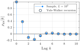
Numerical check. For \(h_1=0.5\) and \(h_2=-0.3\) the closed forms give \(\rho _{\byy }[1]=0.385\), \(\rho _{\byy }[2]=-0.108\) and \(P_y=1.290\). A record of \(L=10^5\) samples gives

h1 = 0.5; h2 = -0.3; L = 1e5;
rng(0); e = randn(L,1);
y = filter(1, [1 -h1 -h2], e);    % the AR(2) model
r = xcorr(y, 2, 'biased');        % lags -2..2, sums divided by L
rho = r(3:5)/r(3)                 % 1, 0.388, -0.106
Py    = r(3)                      % 1.286

within \(1\%\) of the closed forms. The sample ACF follows the recursion of part (c) at every lag, as the figure below shows.

Bibliography

• [1]  Tomas Andersson. Selected topics in frequency estimation. PhD thesis, KTH Royal Institute of Technology, 2003.

• [2]  Dima Bykhovsky. Experimental lognormal modeling of harmonics power of switched-mode power supplies. Energies, 15(2), 2022.

• [3]  Dima Bykhovsky and Asaf Cohen. Electrical network frequency (ENF) maximum-likelihood estimation via a multitone harmonic model. IEEE Transactions on Information Forensics and Security, 8(5):744–753, 2013.

• [4]  Lorenzo Ciampiconi, Adam Elwood, Marco Leonardi, Ashraf Mohamed, and Alessandro Rozza. A survey and taxonomy of loss functions in machine learning. arXiv preprint arXiv:2301.05579, 2023.

• [5]  Angus Dempster, François Petitjean, and Geoffrey I Webb. Rocket: exceptionally fast and accurate time series classification using random convolutional kernels. Data Mining and Knowledge Discovery, 34(5):1454–1495, 2020.

• [6]  Angus Dempster, Daniel F Schmidt, and Geoffrey I Webb. Minirocket: A very fast (almost) deterministic transform for time series classification. In Proceedings of the 27th ACM SIGKDD conference on knowledge discovery & data mining, pages 248–257, 2021.

• [7]  Bo Diao, Kun Wen, Jian Chen, Yueping Liu, Zilin Yuan, Chao Han, Jiahui Chen, Yuxian Pan, Li Chen, Yunjie Dan, Jing Wang, Yongwen Chen, Guohong Deng, Hongwei Zhou, and Yuzhang Wu. Diagnosis of acute respiratory syndrome coronavirus 2 infection by detection of nucleocapsid protein. medRxiv, 2020.

• [8]  Sharon Gannot, Zheng-Hua Tan, Martin Haardt, Nancy F Chen, Hoi-To Wai, Ivan Tashev, Walter Kellermann, and Justin Dauwels. Data science education: The signal processing perspective [sp education]. IEEE Signal Processing Magazine, 40(7):89–93, 2023.

• [9]  Toni Giorgino. Computing and visualizing dynamic time warping alignments in r: the dtw package. Journal of statistical Software, 31:1–24, 2009.

• [10]  Monson H Hayes. Statistical Digital Signal Processing and Modeling. John Wiley & Sons, 1996.

• [11]  Kaiming He, Xiangyu Zhang, Shaoqing Ren, and Jian Sun. Delving deep into rectifiers: Surpassing human-level performance on imagenet classification. In Proceedings of the IEEE international conference on computer vision, pages 1026–1034, 2015.

• [12]  Steven M. Kay. Fundamentals of Statistical Signal Processing, Volume I: Estimation Theory. Prentice Hall, 1993.

• [13]  Nitish Shirish Keskar, Dheevatsa Mudigere, Jorge Nocedal, Mikhail Smelyanskiy, and Ping Tak Peter Tang. On large-batch training for deep learning: Generalization gap and sharp minima. arXiv preprint arXiv:1609.04836, 2017.

• [14]  Jason Lines, Sarah Taylor, and Anthony Bagnall. Hive-cote: The hierarchical vote collective of transformation-based ensembles for time series classification. In 2016 IEEE 16th international conference on data mining (ICDM), pages 1041–1046. IEEE, 2016.

• [15]  Boaz Porat. Digital processing of random signals: theory and methods. Courier Dover Publications, 2008.

• [16]  Pavel Senin and Sergey Malinchik. Sax-vsm: Interpretable time series classification using sax and vector space model. In 2013 IEEE 13th international conference on data mining, pages 1175–1180. IEEE, 2013.

• [17]  Albert Wong, Athena Nguyen, Eugene Li, Yew-Wei Lim, Mike Wu, and Shuk Wai Tsang. Combining classifiers for improved accuracies -voting and linearly weighted algorithms, Feb 2026.

• [18]  Lexiang Ye and Eamonn Keogh. Time series shapelets: a new primitive for data mining. In Proceedings of the 15th ACM SIGKDD international conference on Knowledge discovery and data mining, pages 947–956, 2009.