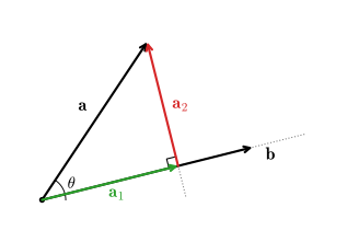
where \(\theta \) is the angle between them. In particular, \(\ba \perp \bb \;\Leftrightarrow \; \theta = 90^\circ \;\Leftrightarrow \; \ba ^T\bb = 0\).
B.1.3 Pseudo-inverse
When \(\bX \in \mathbb {R}^{M\times N}\) has full column rank (\(M \ge N\) and the columns are linearly independent), the matrix \(\bX ^T\bX \) is invertible and the (left, Moore-Penrose) pseudo-inverse is
Definition.
Let \(\bA \in \mathbb {R}^{n\times n}\). A non-zero vector \(\bv \in \mathbb {R}^n\) is an eigenvector of \(\bA \) with associated eigenvalue \(\lambda \in \mathbb {R}\) if
Assume \(\bA \) has \(n\) linearly independent eigenvectors \(\bv _1, \bv _2, \ldots , \bv _n\) (this assumption, called diagonalisability, is non-trivial; not every square matrix satisfies it). Stack them as the columns of
where \(\bm {\Lambda }=\diag (\lambda _1, \lambda _2, \ldots , \lambda _n)\). Multiplying on the right by \(\bQ ^{-1}\) gives the eigendecomposition of \(\bA \),
When \(\bA \) is real symmetric, \(\bA = \bA ^T\), the eigendecomposition always exists and has stronger properties: the eigenvalues \(\lambda _i\) are real, and the eigenvectors \(\bv _i\) can be chosen orthonormal. In that case \(\bQ \)
is an orthogonal matrix, \(\bQ ^{-1} = \bQ ^T\), and
A sample covariance matrix is symmetric and positive semi-definite, so its eigendecomposition has real non-negative eigenvalues and orthonormal eigenvectors.
Positive (semi-)definite matrices
A real symmetric matrix \(\bA \in \mathbb {R}^{n\times n}\) is called
•positive definite (PD), written \(\bA \succ 0\), if \(\bx ^T\bA \bx > 0\) for every non-zero \(\bx \in \mathbb {R}^n\);
•positive semi-definite (PSD), written \(\bA \succeq 0\), if \(\bx ^T\bA \bx \ge 0\) for every \(\bx \in \mathbb {R}^n\) (equality is allowed for non-zero \(\bx \)).
Equivalent characterisations in terms of the eigenvalues \(\lambda _1,\ldots ,\lambda _n\) (which are real because \(\bA \) is symmetric):
• \(\bA \succ 0 \;\Leftrightarrow \; \lambda _i > 0\) for all \(i\);
• \(\bA \succeq 0 \;\Leftrightarrow \; \lambda _i \ge 0\) for all \(i\).
A PD matrix is invertible (none of its eigenvalues is zero); a PSD matrix may be singular. Common examples:
• For any matrix \(\bX \), the Gram matrix \(\bX ^T\bX \) is PSD; it is PD when \(\bX \) has full column rank.
• A sample covariance matrix is PSD; it is PD when the data spans the full feature space.
• The Hessian of a strictly convex function is PD at every point; the Hessian of a convex function is PSD.
Negative definite (\(\bA \prec 0\)) and negative semi-definite (\(\bA \preceq 0\)) are defined analogously, with all eigenvalues strictly negative or non-positive.
B.1.6 Projections
Vector projection
The vector projection of \(\ba \) onto \(\bb \) is the orthogonal projection of \(\ba \) onto the direction of \(\bb \) (Fig. B.2). With \(\hat \bb = \bb /\norm {\bb }\) the
unit vector in the direction of \(\bb \),
Figure B.2: \(\ba _1\) is the projection of \(\ba \) onto \(\bb \).
Subspace projection
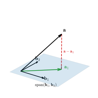
The projection of a vector \(\ba \in \mathbb {R}^N\) onto a subspace spanned by the columns of \(\bB = [\bb _1,\,\bb _2,\,\ldots ,\,\bb _k]\in \mathbb {R}^{N\times k}\) (Fig. B.3) is
where \(\bP \) is the orthogonal projection matrix onto the column space of \(\bB \). It satisfies \(\bP ^2 = \bP \) and \(\bP ^T = \bP \). The single-vector formula above is the special case \(k=1\).
Figure B.3: Orthogonal projection of \(\ba \) onto the subspace spanned by \(\bb _1,\bb _2\).
Condition number
The condition number of a matrix measures how much small perturbations of the input can be amplified in the output of a linear system. For a non-singular matrix \(\bA \),
\(\seteqnumber{0}{B.}{18}\)
\begin{align}
\label {app-math-poor-coditioning} \kappa (\bA ) &= \frac {\sigma _{\max }(\bA )}{\sigma _{\min }(\bA )},\\ \kappa (\bA ^T\bA ) &= \kappa (\bA )^2,
\end{align}
where \(\sigma _{\max }\) and \(\sigma _{\min }\) are the largest and smallest singular values of \(\bA \). For a symmetric positive-definite \(\bA \), the singular values coincide with the absolute eigenvalues, so \(\kappa (\bA ) =
|\lambda _{\max }|/|\lambda _{\min }|\). A large condition number indicates that the matrix is close to singular, leading to numerical inaccuracies in matrix calculations; in particular, forming \(\bA ^T\bA \) (as in the normal equations)
squares the condition number, which is one reason SVD-based solvers are preferred for ill-conditioned least-squares problems.
The indicator \(\indFunc [\text {predicate}]\) equals \(1\) when the predicate is true and \(0\) otherwise. Two notational patterns recur throughout the book.
B.2.1 Sum of a single indicator
Given labels \(Y_1,\ldots ,Y_M\) and a fixed class \(c\), the expression
turns the label vector into a column of 0s and 1s, with a 1 in row \(i\) whenever \(Y_i=c\), and then adds those entries. The sum is simply the number of 1s in that column, i.e. the count of samples whose label is \(c\).
B.2.2 Sum of a product of indicators
A product of two indicators is itself an indicator of the conjunction,
reads two 0/1 columns row by row, multiplies entry by entry, and counts the rows where both columns held a 1. It is the number of samples whose true class is \(c\) and whose predicted class is \(c'\).
The entry-by-entry product of two vectors is called the Hadamard product and written with \(\odot \): if \(\bv ,\bu \in \{0,1\}^M\) are the two indicator columns, then \((\bv \odot \bu )_i = v_i u_i\), and the sum above is
the total of the entries of \(\bv \odot \bu \).
Example B.1: With \(M=5\), true labels \(\bY =(c,\, c,\, b,\, c,\, a)\) and predictions \(\hat \bY =(c,\, b,\,
b,\, c,\, b)\), taking \(c\) as the positive class and asking “true \(c\) predicted as \(c\)”:
The single-indicator column sums give the marginal counts (3 true \(c\), 2 predicted \(c\)); the product column counts samples in both at once (2 correctly predicted as \(c\)).
This is the mechanism behind confusion-matrix entries such as Eq. (17.24) and the agreement-matrix entries in Sec. 19.3.2.
B.3 Function analysis
B.3.1 Minimum, maximum, argmin, argmax
For a real-valued function \(f(x)\):
• \(\min _x f(x)\) is the smallest value attained by \(f\) over all possible \(x\).
• \(\argmin _x f(x)\) is the location where that minimum is attained: if \(y = \argmin _x f(x)\), then \(f(y) = \min _x f(x)\).
The pair \(\max _x f(x)\) and \(\argmax _x f(x)\) are defined analogously. The distinction matters in optimisation: a learning algorithm reports the argmin (the parameter values), not the min (the residual loss).
B.3.2 Vector and matrix calculus
For a scalar-valued function \(f:\mathbb {R}^N \to \mathbb {R}\) of a vector \(\bz = [z_1,\ldots ,z_N]^T\), the gradient is the column vector of partial derivatives,
At a stationary point (\(\nabla _\bz f = \bZero \)), the function has a local minimum if \(\bH \) is positive definite, a local maximum if \(\bH \) is negative definite, and a saddle point if \(\bH \) has eigenvalues of both signs.