Machine Learning & Signals Learning

B Essential formulas

B.1 Linear algebra

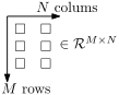
B.1.1 Basic operations

For a column vector \(\bz = [z_1,\,z_2,\,\ldots ,\,z_N]^T \in \mathbb {R}^N\), the squared Euclidean norm is

\begin{equation} \norm {\bz }^2 = \bz ^T\bz = z_1^2 + z_2^2 + \cdots + z_N^2. \end{equation}

For matrices \(\bA \) and \(\bB \) of compatible sizes, the transpose of a product is

\begin{equation} (\bA \bB )^T = \bB ^T\bA ^T. \end{equation}

B.1.2 Dot product

For two vectors \(\ba , \bb \in \mathbb {R}^N\),

\begin{equation} \ba \cdot \bb = \ba ^T\bb = \bb ^T\ba = \norm {\ba }\,\norm {\bb }\,\cos \theta , \end{equation}

where \(\theta \) is the angle between them. In particular, \(\ba \perp \bb \;\Leftrightarrow \; \theta = 90^\circ \;\Leftrightarrow \; \ba ^T\bb = 0\).

B.1.3 Pseudo-inverse

When \(\bX \in \mathbb {R}^{M\times N}\) has full column rank (\(M \ge N\) and the columns are linearly independent), the matrix \(\bX ^T\bX \) is invertible and the (left, Moore-Penrose) pseudo-inverse is

\begin{equation} \bX ^+ = \left (\bX ^T\bX \right )^{-1}\bX ^T, \end{equation}

which satisfies \(\bX ^+\bX = \bI \) and provides the least-squares solution to overdetermined linear systems.

B.1.4 Least squares

The least-squares loss for a linear model \(\bX \bw \approx \bY \) is

\begin{align} \loss (\bw ) &= \norm {\bY -\bX \bw }^2 = (\bY -\bX \bw )^T(\bY -\bX \bw ) \\ &= \bY ^T\bY - 2\bw ^T\bX ^T\bY + \bw ^T\bX ^T\bX \bw . \end{align} Setting the gradient to zero,

\begin{equation} \frac {\partial \loss (\bw )}{\partial \bw } = -2\bX ^T\bY + 2\bX ^T\bX \bw = \bZero , \end{equation}

gives the normal equations \(\bX ^T\bX \bw = \bX ^T\bY \) and the closed-form solution

\begin{equation} \bw ^\star = \left (\bX ^T\bX \right )^{-1}\bX ^T\bY = \bX ^+\bY . \end{equation}

B.1.5 Eigenvalues and eigenvectors

Definition. Let \(\bA \in \mathbb {R}^{n\times n}\). A non-zero vector \(\bv \in \mathbb {R}^n\) is an eigenvector of \(\bA \) with associated eigenvalue \(\lambda \in \mathbb {R}\) if

\begin{equation} \bA \bv = \lambda \bv . \end{equation}

Geometrically, \(\bA \) acts on any vector along the direction of \(\bv \) by scaling it by the factor \(\lambda \), without rotation.

The eigenvalues of \(\bA \) satisfy the identities

\begin{align} \operatorname {tr}(\bA ) &= \sum _{i=1}^n a_{ii} = \sum _{i=1}^n \lambda _i,\\ \det (\bA ) &= \prod _{i=1}^n \lambda _i. \end{align}

Eigendecomposition

Assume \(\bA \) has \(n\) linearly independent eigenvectors \(\bv _1, \bv _2, \ldots , \bv _n\) (this assumption, called diagonalisability, is non-trivial; not every square matrix satisfies it). Stack them as the columns of

\begin{equation} \bQ = \begin{bmatrix} \bv _1 & \bv _2 & \cdots & \bv _n \end {bmatrix}. \end{equation}

Applying \(\bA \) to each column scales it by the corresponding eigenvalue, so column-by-column

\begin{equation} \bA \bQ = \begin{bmatrix} \lambda _1\bv _1 & \lambda _2\bv _2 & \cdots & \lambda _n\bv _n \end {bmatrix} = \bQ \bm {\Lambda }, \end{equation}

where \(\bm {\Lambda }=\diag (\lambda _1, \lambda _2, \ldots , \lambda _n)\). Multiplying on the right by \(\bQ ^{-1}\) gives the eigendecomposition of \(\bA \),

\begin{align} \bA &= \bQ \bm {\Lambda }\bQ ^{-1},\\ \bQ ^{-1}\bA \bQ &= \bm {\Lambda }. \end{align}

Symmetric case (spectral theorem)

When \(\bA \) is real symmetric, \(\bA = \bA ^T\), the eigendecomposition always exists and has stronger properties: the eigenvalues \(\lambda _i\) are real, and the eigenvectors \(\bv _i\) can be chosen orthonormal. In that case \(\bQ \) is an orthogonal matrix, \(\bQ ^{-1} = \bQ ^T\), and

\begin{equation} \bA = \bQ \bm {\Lambda }\bQ ^T. \end{equation}

A sample covariance matrix is symmetric and positive semi-definite, so its eigendecomposition has real non-negative eigenvalues and orthonormal eigenvectors.

Positive (semi-)definite matrices

A real symmetric matrix \(\bA \in \mathbb {R}^{n\times n}\) is called

• • positive definite (PD), written \(\bA \succ 0\), if \(\bx ^T\bA \bx > 0\) for every non-zero \(\bx \in \mathbb {R}^n\);

• • positive semi-definite (PSD), written \(\bA \succeq 0\), if \(\bx ^T\bA \bx \ge 0\) for every \(\bx \in \mathbb {R}^n\) (equality is allowed for non-zero \(\bx \)).

Equivalent characterisations in terms of the eigenvalues \(\lambda _1,\ldots ,\lambda _n\) (which are real because \(\bA \) is symmetric):

• • \(\bA \succ 0 \;\Leftrightarrow \; \lambda _i > 0\) for all \(i\);

• • \(\bA \succeq 0 \;\Leftrightarrow \; \lambda _i \ge 0\) for all \(i\).

A PD matrix is invertible (none of its eigenvalues is zero); a PSD matrix may be singular. Common examples:

• • For any matrix \(\bX \), the Gram matrix \(\bX ^T\bX \) is PSD; it is PD when \(\bX \) has full column rank.

• • A sample covariance matrix is PSD; it is PD when the data spans the full feature space.

• • The Hessian of a strictly convex function is PD at every point; the Hessian of a convex function is PSD.

Negative definite (\(\bA \prec 0\)) and negative semi-definite (\(\bA \preceq 0\)) are defined analogously, with all eigenvalues strictly negative or non-positive.

B.1.6 Projections

Vector projection

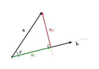
The vector projection of \(\ba \) onto \(\bb \) is the orthogonal projection of \(\ba \) onto the direction of \(\bb \) (Fig. B.2). With \(\hat \bb = \bb /\norm {\bb }\) the unit vector in the direction of \(\bb \),

\begin{equation} \ba _1 = (\ba \cdot \hat \bb )\,\hat \bb = \frac {\ba ^T\bb }{\norm {\bb }^2}\,\bb . \end{equation}

Subspace projection

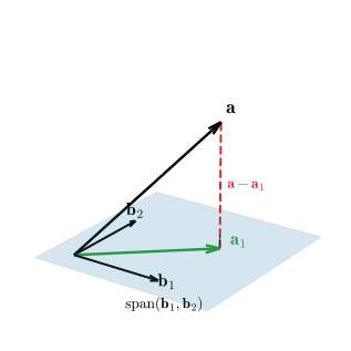
The projection of a vector \(\ba \in \mathbb {R}^N\) onto a subspace spanned by the columns of \(\bB = [\bb _1,\,\bb _2,\,\ldots ,\,\bb _k]\in \mathbb {R}^{N\times k}\) (Fig. B.3) is

\begin{equation} \ba _1 = \bP \ba , \qquad \bP = \bB (\bB ^T\bB )^{-1}\bB ^T, \end{equation}

where \(\bP \) is the orthogonal projection matrix onto the column space of \(\bB \). It satisfies \(\bP ^2 = \bP \) and \(\bP ^T = \bP \). The single-vector formula above is the special case \(k=1\).

Condition number

The condition number of a matrix measures how much small perturbations of the input can be amplified in the output of a linear system. For a non-singular matrix \(\bA \),

\begin{align} \label {app-math-poor-coditioning} \kappa (\bA ) &= \frac {\sigma _{\max }(\bA )}{\sigma _{\min }(\bA )},\\ \kappa (\bA ^T\bA ) &= \kappa (\bA )^2, \end{align} where \(\sigma _{\max }\) and \(\sigma _{\min }\) are the largest and smallest singular values of \(\bA \). For a symmetric positive-definite \(\bA \), the singular values coincide with the absolute eigenvalues, so \(\kappa (\bA ) = |\lambda _{\max }|/|\lambda _{\min }|\). A large condition number indicates that the matrix is close to singular, leading to numerical inaccuracies in matrix calculations; in particular, forming \(\bA ^T\bA \) (as in the normal equations) squares the condition number, which is one reason SVD-based solvers are preferred for ill-conditioned least-squares problems.

For example,

\begin{equation} \bA = \begin{bmatrix} 1 & 1 & -\epsilon \\ \epsilon & 0 & 1 \\ 0 & \epsilon & 1 \end {bmatrix} \;\Rightarrow \; \kappa (\bA )\approx \sqrt {2}/\epsilon ,\quad \kappa (\bA ^T\bA )\approx 2/\epsilon ^2. \end{equation}

B.2 Indicator functions and counting

The indicator \(\indFunc [\text {predicate}]\) equals \(1\) when the predicate is true and \(0\) otherwise. Two notational patterns recur throughout the book.

B.2.1 Sum of a single indicator

Given labels \(Y_1,\ldots ,Y_M\) and a fixed class \(c\), the expression

\begin{equation} \sum _{i=1}^{M} \indFunc [Y_i = c] \end{equation}

turns the label vector into a column of 0s and 1s, with a 1 in row \(i\) whenever \(Y_i=c\), and then adds those entries. The sum is simply the number of 1s in that column, i.e. the count of samples whose label is \(c\).

B.2.2 Sum of a product of indicators

A product of two indicators is itself an indicator of the conjunction,

\begin{equation} \indFunc [A]\,\indFunc [B] = \indFunc [A \text { and } B], \end{equation}

because the product is \(1\) only when both factors are \(1\). For two label vectors (say the truth \(Y_i\) and a prediction \(\hat Y_i\)), the sum

\begin{equation} \sum _{i=1}^{M} \indFunc [Y_i = c]\,\indFunc [\hat Y_i = c'] \end{equation}

reads two 0/1 columns row by row, multiplies entry by entry, and counts the rows where both columns held a 1. It is the number of samples whose true class is \(c\) and whose predicted class is \(c'\).

The entry-by-entry product of two vectors is called the Hadamard product and written with \(\odot \): if \(\bv ,\bu \in \{0,1\}^M\) are the two indicator columns, then \((\bv \odot \bu )_i = v_i u_i\), and the sum above is the total of the entries of \(\bv \odot \bu \).

This is the mechanism behind confusion-matrix entries such as Eq. (12.24) and the agreement-matrix entries in Sec. 14.3.2.

B.3 Function analysis

B.3.1 Minimum, maximum, argmin, argmax

For a real-valued function \(f(x)\):

• • \(\min _x f(x)\) is the smallest value attained by \(f\) over all possible \(x\).

• • \(\argmin _x f(x)\) is the location where that minimum is attained: if \(y = \argmin _x f(x)\), then \(f(y) = \min _x f(x)\).

The pair \(\max _x f(x)\) and \(\argmax _x f(x)\) are defined analogously. The distinction matters in optimisation: a learning algorithm reports the argmin (the parameter values), not the min (the residual loss).

B.3.2 Vector and matrix calculus

For a scalar-valued function \(f:\mathbb {R}^N \to \mathbb {R}\) of a vector \(\bz = [z_1,\ldots ,z_N]^T\), the gradient is the column vector of partial derivatives,

\begin{equation} \nabla _\bz f(\bz ) = \begin{bmatrix} \dfrac {\partial f}{\partial z_1} \\[5pt] \dfrac {\partial f}{\partial z_2} \\ \vdots \\ \dfrac {\partial f}{\partial z_N} \end {bmatrix} \in \mathbb {R}^N. \end{equation}

The Hessian is the symmetric \(N\times N\) matrix of second partial derivatives,

\begin{equation} \bH = \nabla _\bz ^2 f(\bz ),\qquad H_{ij} = \frac {\partial ^2 f}{\partial z_i\,\partial z_j}. \end{equation}

At a stationary point (\(\nabla _\bz f = \bZero \)), the function has a local minimum if \(\bH \) is positive definite, a local maximum if \(\bH \) is negative definite, and a saddle point if \(\bH \) has eigenvalues of both signs.

B.4 Chi-square distribution

Definition

Let \(Z_1, Z_2, \ldots , Z_k\) be independent standard normal variables, \(Z_i\sim \mathcal {N}(0,1)\). Their sum of squares

\begin{equation} \label {eq-app-chi2-def} Q = \sum _{i=1}^{k} Z_i^2 \end{equation}

follows the chi-square distribution with \(k\) degrees of freedom, written \(Q\sim \chi ^2_k\). Two properties follow directly from (B.27): \(Q\ge 0\), because it is a sum of squares, and the parameter \(k\) is nothing more than the number of independent squared terms being added.

The probability density function is

\begin{equation} f(q;k) = \frac {1}{2^{k/2}\,\Gamma (k/2)}\,q^{k/2-1}e^{-q/2},\qquad q>0, \end{equation}

where \(\Gamma (\cdot )\) is the gamma function. The density is right-skewed, and the skew decreases as \(k\) grows.

Moments,

\begin{align} \E [Q] &= k,\\ \Var [Q] &= 2k. \end{align}

For independent \(Q_1\sim \chi ^2_{k_1}\) and \(Q_2\sim \chi ^2_{k_2}\),

\begin{equation} Q_1 + Q_2 \sim \chi ^2_{k_1+k_2}. \end{equation}

The degrees of freedom add exactly as the squared terms of (B.27) do. Combined with the central limit theorem, this also explains the large-\(k\) behavior: a \(\chi ^2_k\) variable is a sum of \(k\) independent contributions, so

\begin{equation} Q \;\approx \; \mathcal {N}(k,\,2k), \qquad k \gg 1. \end{equation}

Upper-tail quantiles

The upper-tail quantile \(\chi ^2_{k,\,1-\alpha }\) is the value that a \(\chi ^2_k\) variable exceeds with probability \(\alpha \),

\begin{equation} \label {eq-app-chi2-quantile} \Pr \left (Q > \chi ^2_{k,\,1-\alpha }\right ) = \alpha , \qquad Q\sim \chi ^2_k , \end{equation}

the subscript naming the cumulative level \(1-\alpha \) rather than the tail left above it. It is computed numerically in general; two cases are closed form.

By (B.27) a \(\chi ^2_1\) variable is \(Z^2\) with \(Z\sim \mathcal {N}(0,1)\), so its quantile is a two-sided normal threshold squared,

\begin{equation} \label {eq-app-chi2-quantile-1} \chi ^2_{1,\,1-\alpha } = \left [\Phi ^{-1}\left (1-\alpha /2\right )\right ]^2 , \end{equation}

which returns \(3^2 = 9\) at \(\alpha = 0.0027\). For \(k=2\) the density reduces to \(f(q;2) = \tfrac {1}{2}e^{-q/2}\), so the tail and its inverse are elementary,

\begin{equation} \label {eq-app-chi2-tail-2} \Pr \left (\chi ^2_2 > \tau \right ) = e^{-\tau /2} , \qquad \chi ^2_{2,\,1-\alpha } = -2\ln \alpha . \end{equation}

Sum of squared deviations For an i.i.d. Gaussian sample \(X_1,\ldots ,X_n\sim \mathcal {N}(\mu ,\sigma ^2)\), the sum of squared deviations around the sample mean \(\bar X\) satisfies

\begin{equation} \frac {1}{\sigma ^2}\sum _{i=1}^{n}\left (X_i-\bar X\right )^2 \sim \chi ^2_{n-1}. \end{equation}

One degree of freedom is lost because the mean was estimated from the same data: the \(n\) deviations are constrained by \(\sum _i (X_i-\bar X)=0\), leaving only \(n-1\) of them free. Together with \(\Var [Q]=2k\) this is what makes the variance of an estimated variance proportional to \(2/n\).