Machine Learning & Signals Learning
21 ARMA Model
This chapter extends least-squares (LS)-based modeling to systems and time-series contexts, focusing on linear prediction coefficients derived from signals. Instead of restricting to a predefined parametric form like a sinusoid, here we consider arbitrary zero-mean finite-time signals \(x[n]\) and \(y[n], n=0,\ldots , L-1\), in the presence of zero-mean noise, \(\epsilon [n]\).
21.1 Auto-Correlation Function
21.1.1 AR(1)
In system modeling and time-series analysis, a common approach is to express the current sample of a signal in terms of its past values. A simple first-order autoregressive (AR(1)) model predicts the current sample \(x[n]\) from a single past sample \(x[n-1]\), using the system model
\(\seteqnumber{0}{}{0}\)\begin{equation} \label {eq:ar1} x[n]=h_1x[n-1] + \epsilon [n]. \end{equation}
and
\(\seteqnumber{0}{}{1}\)\begin{equation} \hat {x}[n] = h_1x[n-1] \end{equation}
Here, \(h_1\) is the linear prediction coefficient that indicates how strongly the previous sample \(x[n-1]\) influences the current sample \(x[n]\).
To determine \(h_1\), minimization of SE loss function
\(\seteqnumber{0}{}{2}\)\begin{equation} \loss (h_1) = \sum _n \left (x[n] - h_1x[n-1])\right )^2 \end{equation}
is used. Setting the derivative of \(\loss (h_1)\) with respect to \(h_1\) to zero leads to
\(\seteqnumber{0}{}{3}\)\begin{equation} \label {eq-a1} \frac {d\mathcal {L}(a)}{da} =2\sum _n (x[n]-h_1x[n-1])(-x[n-1])=0 \end{equation}
Finally, the LS solution for \(h_1\) is
\(\seteqnumber{0}{}{4}\)\begin{equation} \label {eq-acf-a1} h_1 = \frac {\sum _n x[n]x[n-1]}{\sum _n x^2[n-1]}. \end{equation}
The value \(h_1\) is termed as the (single) prediction coefficient of AR(1) model.
Matrix formulation
The coefficient may be formulated as a relation between two vectors
\(\seteqnumber{0}{}{5}\)\begin{equation} \label {eq:ar1:matrix} \hat {\by }= \begin{bmatrix} x[1] \\ x[2] \\ \vdots \\ x[L-2]\\ x[L-1] \end {bmatrix} \quad \bx = \begin{bmatrix} x[0]\\ x[1] \\ \vdots \\ x[L-3] \\ x[L-2] \end {bmatrix}, \end{equation}
such that
\(\seteqnumber{0}{}{6}\)\begin{equation} \hat {\by } = h_1 \bx . \end{equation}
The correspoding MMSE loss is
\(\seteqnumber{0}{}{7}\)\begin{equation} \loss (h_1) = \norm {\by - h_1 \bx }^2 \end{equation}
and its minimum is given by normal equation, (Eq. (3.5)),
\(\seteqnumber{0}{}{8}\)\begin{equation} \label {eq:normal_eq_vector} h_1 = {\left (\bx ^T\bx \right )^{-1}}\bx ^T\by . \end{equation}
The substitution results in the solution identical to Eq. (21.5).
Prediction with \(k\)-samples difference
To generalize beyond a single lag, we use one-coefficient prediction from the current sample \(x[n]\) and its time-shifted version \(x[n-k]\), using the \(k\)-step predictor,
\(\seteqnumber{0}{}{9}\)\begin{equation} \hat {x}[n]=h_kx[n-k]. \end{equation}
The corresponding solution is very similar to the solution for \(k=1\),
\(\seteqnumber{0}{}{10}\)\begin{equation} \label {eq-acf-ak} h_k = \frac {\sum _n x[n]x[n-k]}{\sum _n x^2[n-k]}. \end{equation}
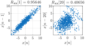
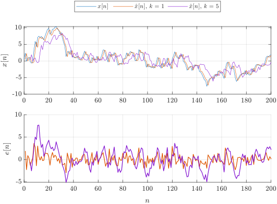
The linear dependence between \(x[n]\) and \(x[n-k]\), and the prediction it enables, are illustrated in Fig. 21.1 for an AR(1) signal. The dependence weakens as the lag grows, and with it the accuracy of the prediction.
21.1.2 Auto-correlation function (ACF)
The nominator of Eq. (21.11) is termed (raw, or unscaled) auto-correlation function (ACF) at lag \(k\),
\(\seteqnumber{0}{}{11}\)\begin{equation} R_{\bx \bx }[k] = \sum _n x[n]x[n-k],\quad k=0,\ldots ,L-1 \end{equation}
The ACF provides a measure of how linearly dependent the signal is on its shifted versions. Variants like biased, unbiased, and normalized ACF offer different normalization schemes to handle finite data length and scaling issues.
The signal energy is given by
\(\seteqnumber{0}{}{12}\)\begin{equation} \label {eq:arma:energy} E_\bx = \sum _{n=0}^{L-1} x^2[n] = R_\bxx [0] \end{equation}
Biased auto-correlation Another useful definition is averaged sum of \(y[n]y[n-k]\),
\(\seteqnumber{0}{}{13}\)\begin{equation} \label {eq-acf-biased} \begin{aligned} R_{\bx \bx ,biased}[k] &= \frac {1}{L}\sum _n x[n]x[n-k],\quad k=0,\ldots ,L-1\\ &= \frac {1}{L}R_{\bx \bx }[k] \end {aligned} \end{equation}
is termed biased (see Sec. 1.1.3 for bias definition) ACF. The corresponding average power is given by
\(\seteqnumber{0}{}{14}\)\begin{equation} P_\bx = \frac {1}{L}\sum _n x^2[n] = R_{\bxx ,biased}[0] \end{equation}
Normalized auto-correlation Another version is normalized ACF of the form
\(\seteqnumber{0}{}{15}\)\begin{equation} \label {eq-acf-norm} R_{\bx \bx ,norm}[k] = \frac {R_{\bx \bx }[k]}{R_{\bx \bx }[0]}\lesssim h_k. \end{equation}
Note, the difference between denominator above and the one in Eq. (21.11) (where the lagged sum runs over \(n=k,\ldots ,L-1\)) is
\(\seteqnumber{0}{}{16}\)\begin{equation} \sum _{n=0}^{L-1} x^2[n] - \sum _{n=k}^{L-1}x^2[n-k] = x^2[L-k] + \cdots + x^2[L-1], \end{equation}
i.e. the last \(k\) samples of the squared signal. Under stationarity and \(k\ll L\), these boundary terms are negligible relative to \(R_{\bxx }[0]\), so \(h_k\) in Eq. (21.11) and \(R_{\bxx ,norm}[k]\) are approximately equal for a sufficiently high \(L\). Moreover, here the denominator is \(k\)-independent.
Unbiased auto-correlation Note, that the ACF includes summation only of \(n-k\) terms. Another useful normalization is
\(\seteqnumber{0}{}{17}\)\begin{equation} \label {eq-acf-unbiased} \begin{aligned} R_{\bx \bx ,unbiased}[k] &= \frac {1}{L-k}\sum _n x[n]x[n-k]\\ &= \frac {1}{L-k}R_{\bx \bx }[k] \end {aligned} \end{equation}
This time it is assumed that
\(\seteqnumber{0}{}{18}\)\begin{equation} \label {eq:acf-stationarity} \begin{aligned} \frac {1}{L}\sum _n x^2[n] &\approx \frac {1}{L-k}\sum _n x^2[n-k]\\ \frac {x^2[0] +x^2[1] + \cdots x^2[L-1]}{L} &\approx \frac {x^2[k] + \cdots x^2[L-1]}{L-k} \end {aligned} \end{equation}
and the resulting expression
\(\seteqnumber{0}{}{19}\)\begin{equation} \begin{aligned} \frac {L}{L-k}\frac {R_{\bx \bx }[k]}{R_{\bx \bx }[0]}=\frac {L}{L-k}R_{\bx \bx ,norm}[k]\\ =\frac {R_{\bx \bx ,unbiased}[k]}{R_{\bx \bx ,unbiased}[0]} \approx h_k \end {aligned} \end{equation}
is assumed to be closer approximation to \(h_k\) than the normalized auto-correlation, for a relatively small values of \(k\).
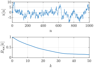
An AR(1) signal and its normalized ACF are shown in Fig. 21.2. The ACF starts at \(R_{\bxx ,norm}[0]=1\) and decays with the lag, reproducing the loss of predictability seen in Fig. 21.1.
Correlation time The correlation time, \(k_c\) is the lag where \(R_{\bxx ,norm}[k_c]\) falls below a threshold,
\(\seteqnumber{0}{}{20}\)\begin{equation} \label {eq-correlation-time} R_{\bxx ,norm}[k_c] = 0.5 \text { or } 0.1 \text { or }\exp (-1) \end{equation}
The predictability is assumed negligible for \(k>k_c\),
\(\seteqnumber{0}{}{21}\)\begin{equation} \label {eq-correlation-time-limit} R_{\bxx ,norm}[k>k_c]\approx 0 \end{equation}
The decision threshold depends on the field of application. For example, one of the most applicable ACF for natural processes is
\(\seteqnumber{0}{}{22}\)\begin{equation} R_{\bxx ,norm}[k] = \exp (-\frac {k}{k_c}) \end{equation}
with \(R_{\bxx ,norm}[k_c] = \exp (-1)\).
Note, correlation time is mostly used in physics and engineering models and is less applicable in social sciences.
Correlation Coefficient Interpretation
All normalizations above still depend on the amplitude of the signal: replacing \(x[n]\) by \(ax[n]\) multiplies \(R_{\bxx }[k]\) by \(a^2\). Comparing the predictability of two different signals, or of the same signal recorded at a different gain, therefore requires a quantity on a fixed scale. The correlation coefficient achieves this by dividing the raw ACF by the energies of both vectors being compared,
\(\seteqnumber{0}{}{23}\)\begin{equation} \label {eq:corr-coeff-def} \rho _{\bxx }[k] \triangleq \frac {\sum _n x[n]x[n-k]}{\sqrt {\sum _n x^2[n]\,\sum _n x^2[n-k]}} = \frac {R_{\bxx }[k]}{\sqrt {R_{\bxx }[0]\cdot \sum _n x^2[n-k]}}. \end{equation}
The denominator combines both energies involved: \(R_{\bxx }[0]=\sum _n x^2[n]\), the energy of the signal (Eq. (21.13)), and \(\sum _n x^2[n-k]\), the energy of its lagged copy. Taking the square root of their product, instead of dividing by either energy alone, treats the two vectors symmetrically, so that exchanging them leaves \(\rho _{\bxx }[k]\) unchanged. The result is always bounded,
\(\seteqnumber{0}{}{24}\)\begin{equation} \label {eq:rho-bounded} -1\le \rho _{\bxx }[k]\le 1, \end{equation}
where \(\abs {\rho _{\bxx }[k]}=1\) is reached only if \(x[n]\) and \(x[n-k]\) are exactly proportional.
Geometric mean and the Cauchy–Schwarz bound (*) The geometric mean of two non-negative numbers \(a\) and \(b\) is \(\sqrt {ab}\), the multiplicative counterpart of the arithmetic mean \((a+b)/2\). The denominator of Eq. (21.24) is therefore the geometric mean of the two energies, and the bound Eq. (21.25) is the Cauchy–Schwarz inequality applied to \(x[n]\) and \(x[n-k]\).
To prove it, note that for any real \(\lambda \) a sum of squares cannot be negative,
\(\seteqnumber{0}{}{25}\)\begin{equation} \label {eq:cs-quadratic} q(\lambda ) = \sum _n \left (\lambda \,x[n] + x[n-k]\right )^2 = \lambda ^2 R_{\bxx }[0] + 2\lambda \,R_{\bxx }[k] + \sum _n x^2[n-k] \;\ge \; 0 . \end{equation}
Assume \(R_{\bxx }[0]>0\), so that \(q(\lambda )\) is a parabola opening upwards; otherwise \(x[n]\equiv 0\) and \(\rho _{\bxx }[k]\) is undefined. A parabola that is never negative crosses zero at most once, so its discriminant cannot be positive,
\(\seteqnumber{0}{}{26}\)\begin{equation} 4R_{\bxx }^2[k] - 4R_{\bxx }[0]\sum _n x^2[n-k] \;\le \; 0 \quad \Longleftrightarrow \quad \abs {R_{\bxx }[k]} \;\le \; \sqrt {R_{\bxx }[0]\sum _n x^2[n-k]} . \end{equation}
The ACF at any lag therefore never exceeds the geometric mean of the two energies, and dividing by it gives Eq. (21.25).
Reading the value Eq. (21.24) is the sample Pearson correlation coefficient of Sec. 2.2.2, evaluated for the pair of vectors \(x[n]\) and \(x[n-k]\). The mean subtraction appearing there is unnecessary here, because the signal is assumed zero-mean. Its interpretation carries over unchanged: the sign gives the direction of the linear association and the magnitude its strength, with \(\rho _{\bxx }[k]=0\) indicating no linear dependence at that lag. Two points are specific to the lag setting:
-
• Because the amplitude cancels, \(\rho _{\bxx }[k]\) is dimensionless and unaffected by the gain of the recording, so values obtained at different lags and from different records are directly comparable.
-
• Its magnitude fixes the loss achievable by the one-coefficient predictor, as developed in the Model Loss part below.
Relation to the normalized ACF Under the same stationarity assumption used for the unbiased ACF (Eq. (21.19)), \(\sum _n x^2[n-k]\approx \tfrac {L-k}{L}R_{\bxx }[0]\), and
\(\seteqnumber{0}{}{27}\)\begin{equation} \rho _{\bxx }[k] \approx \sqrt {\frac {L}{L-k}}\,R_{\bxx ,norm}[k] \approx R_{\bxx ,norm}[k] \approx h_k \qquad (k\ll L). \end{equation}
The second step drops the factor \(\sqrt {L/(L-k)}\), which tends to \(1\) only for \(k\ll L\). For a short record or a large lag this factor is not negligible, and Eq. (21.24) has to be evaluated directly.
Sample vs. population coefficient
Eq. (21.24) is a sample quantity: it is computed from one finite record of length \(L\), so a different record of the same process yields a slightly different value. The population coefficient is the value it converges to,
\(\seteqnumber{0}{}{28}\)\begin{equation} \label {eq:rho-population} \rho _{\bxx }^{\text {pop}}[k] = \lim _{L\to \infty }\rho _{\bxx }[k], \end{equation}
and it is the quantity that a modeling assumption such as whiteness of the noise actually refers to. In practice the sample \(\rho _{\bxx }[k]\) is used in its place, with \(R_{\bxx ,norm}[k]\) as the stationarity-based approximation.
The summary of the different ACF normalizations and their relation to the prediction coefficient \(h_k\) is given in Table 21.1. The biased and unbiased ACFs keep the scale of the signal, as their value at \(k=0\) shows, so neither is by itself an approximation of the dimensionless \(h_k\); only their ratio to that lag-\(0\) value is comparable with it.
| Quantity | Eq. | Norm. factor | Value at \(k=0\) | Ratio to \(k=0\) value | Relation to \(h_k\) |
| \(R_{\bxx }[k]\) (raw) | (21.11) | none | \(E_\bx \) | \(R_{\bxx ,norm}[k]\) | numerator of \(h_k\) |
| \(R_{\bxx ,biased}[k]\) | (21.14) | \(L\) | \(P_\bx \) | \(R_{\bxx ,norm}[k]\) | only through the ratio |
| \(R_{\bxx ,norm}[k]\) | (21.16) | \(R_{\bxx }[0]\) | \(1\) | \(R_{\bxx ,norm}[k]\) | \(\lesssim h_k\), underestimates for large \(k\) |
| \(R_{\bxx ,unbiased}[k]\) | (21.18) | \(L-k\) | \(P_\bx \) | \(\frac {L}{L-k}R_{\bxx ,norm}[k]\) | \(\approx h_k\) through the ratio |
| \(\rho _{\bxx }[k]\) | (21.24) | geometric mean of energies | \(1\) | \(\rho _{\bxx }[k]\) | \(\approx h_k\) under stationarity, \(\abs {\rho _{\bxx }[k]}\le 1\) |
21.1.3 ACF Properties
The signal energy (21.13) is the highest value of ACF,
\(\seteqnumber{0}{}{29}\)\begin{equation} R_{\bxx }[0] > R_{\bxx }[k]. \end{equation}
Theoretically, \(R_{\bxx }[0] = R_{\bxx }[k]\) may happen under certain conditions but unachievable for the practical time-limited signals.
The ACF has inherent time symmetry (backward prediction),
\(\seteqnumber{0}{}{30}\)\begin{equation} \label {eq:acf_symmetry} R_{\bx \bx }[k] =R_{\bx \bx }[-k] \end{equation}
that reduces the need to recalculation for \(k<0\).
Minimum Loss
In matrix form (by Eq. (3.21)), the loss is given by
\(\seteqnumber{0}{}{31}\)\begin{equation} \loss _{min}(h_k) =\be ^T\be = \by ^T\by - h_k\by ^T\bx \end{equation}
The resulting loss is given by (following Eq. (3.21))
\(\seteqnumber{0}{}{32}\)\begin{equation} \label {eq-signals-min-J} \begin{aligned} \loss _{min}(h_k) &= \sum _{n=0}^{L-1}x^2[n] - h_k\sum _{n=0}^{L-1}x[n]x[n-k]\\[3pt] &= R_{\bx \bx }[0] - h_kR_{\bx \bx }[k]. \end {aligned} \end{equation}
Since \(\sum _n x^2[n-k]\le R_{\bxx }[0]\) implies \(h_k\ge R_{\bxx ,norm}[k]\), the loss is upper-bounded by
\(\seteqnumber{0}{}{33}\)\begin{equation} \loss _{min}(h_k) \le R_{\bx \bx }[0]\left (1-R_{\bx \bx ,norm}^2[k]\right ), \end{equation}
and, under the stationarity approximation \(R_{\bxx ,norm}[k]\approx \rho _{\bxx }[k]\) (Eq. (21.24)),
\(\seteqnumber{0}{}{34}\)\begin{equation} \loss _{min}(h_k) \approx R_{\bx \bx }[0]\left (1-\rho _{\bxx }^2[k]\right ). \end{equation}
The correlation coefficient \(\rho _{\bxx }[k]\) is a measure of linear dependence between \(x[n]\) and \(x[n-k]\).
-
• For noiseless data and a linear relation between the samples, the prediction is perfect, \(\abs {\rho _{\bx \bx }[k]}=1\) and \(\loss _{min}=0\).
-
• Without any linear dependence, \(\rho _{\bx \bx }[k]=h_k=0\) and the resulting prediction is \(\hat {x}[n] = 0\).
This can be summarized as (see also (21.13) for interpretation)
\(\seteqnumber{0}{}{35}\)\begin{equation} \label {eq-ar-loss-bounds} 0\leq \loss _{min}(h_k) \leq R_\bxx [0] \end{equation}
The illustration of the correlation coefficient principles is presented in Fig. 21.1.
MSE and RMSE The corresponding MSE and RMSE metrics are given by
\(\seteqnumber{1}{21.37}{0}\)\begin{align} MSE(h_k) &= \frac {1}{L}\loss _{min}(h_k)\\ RMSE(h_k) &= \sqrt {\frac {1}{L}\loss _{min}(h_k)} \end{align}
21.1.4 Auto-covariance
For simplicity, a zero-average, \(\bar {x}[n]=0\), was assumed. When the signals is non-zero mean, the subtraction of signal average (DC level) from the signal, \(x[n] = x[n]-\bar {x}[n]\) before auto-correlation calculation is termed as auto-covariance.
Note, both auto-correlation and auto-covariance have similar abbreviation, ACF. Typically, ACF is used for auto-correlation, since majority of the signals are zero-mean.
Tip:
-
• ACF calculation may be significantly speed-up with appropriate algorithms and the bounded maximum value of \(k\le k_{max}\). The value of \(k_{max}\) may be decided by Eq. (21.22).
21.2 Power Spectral Density (PSD)
21.2.1 Relation between ACF and PSD
From the signal processing point of view, the interpretation of a DFT of some general random signal is non-trivial. For example, phases \(\theta _k\) of some random origin will be quite different for each time-segment (or realization) of the signal. The Wiener–Khinchin theorem states that the PSD (pages (page for section 20.4.2) and (page for section 20.6.3)) of stationary random signal is the Fourier transform of the ACF. For the raw ACF \(R_{\bxx }[m]\), with \(m\) denoting the lag,
\(\seteqnumber{0}{}{37}\)\begin{equation} \label {eq:wiener-khinchin} S_\bxx [k] = \DFTtr {R_{\bxx }[m]} = \abs {\DFTtr {x[n]}}^2,\quad k=0,\ldots ,N-1 \end{equation}
Transforming the biased ACF instead (Eq. (21.14)) scales the result by \(1/L\) and gives the raw periodogram \(\hat {S}_\bxx [k]=\abs {\DFTtr {x[n]}}^2/L\) used in Sec. 20.7.4; the two differ only by that constant.
Important properties are
-
• \(S_\bxx [k]\in \Re \), due to the symmetry (Eq. (21.31)) of \(R_\bxx [k]\) it results \(\theta _k=0\forall k\).
-
• \(S_\bxx [k]\ge 0\quad \forall k\).
This relation shows, that random signal also includes spectral interpretation.
-
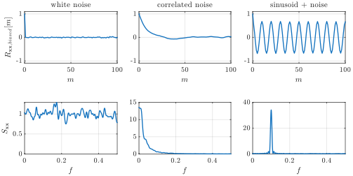
Example 21.1: Three signals of equal power are compared in Fig. 21.3, each with its ACF and the PSD obtained from it.
-
• White noise: the ACF is non-zero only at \(m=0\), and the PSD is flat. A signal that is uncorrelated with its own past spreads its power evenly over all frequencies.
-
• Correlated noise: the ACF decays slowly, and the power concentrates at low frequency. The slower the decay, that is the longer the correlation time (Eq. (21.21)), the narrower the peak.
-
• Sinusoid in noise: the ACF oscillates at the frequency of the sinusoid, and the PSD has a peak there.
Since all three signals carry the same total power, the panels differ only in how that power is spread over frequency.
-
Interpretation
Peaks The PSD shows where (in frequency) the signal has most of its energy. Peaks in the PSD correspond to frequencies at which the signal exhibits strong periodic or quasi-periodic components.
Periodicity Slowly decaying (long-memory) correlations in the time domain often translate into a PSD that has more energy at low frequencies (indicating slow variations in time), as in the center column of Fig. 21.3. Conversely, if the ACF shows periodicity, the PSD will have distinct peaks at the corresponding harmonic frequencies, as in the right column.
Time-shifts The ACF reveals how similar a signal is to itself at different time shifts. A slowly decaying ACF indicates strong long-term correlations, while a rapidly decaying ACF suggests only short-range predictability.
21.2.2 Frequency estimation via ACF peak
For a (quasi-)periodic signal, the ACF \(R_{\bxx }[k]\) inherits the period of \(x[n]\): its largest non-trivial peak appears at the lag corresponding to one signal period. This provides a time-domain alternative to the periodogram-peak estimator of Sec. 20.4.
Using the biased ACF \(R_{\bxx ,biased}[k]\) (Eq. (21.14)), the estimator is
\(\seteqnumber{0}{}{38}\)\begin{equation} \label {eq:freq-acf-estimator} \hat {k}_0 = \arg \max _{k\ge k_{\min }} R_{\bxx ,biased}[k],\quad \hat {F}_0 = \frac {F_s}{\hat {k}_0},\quad \hat {\omega }_0 = \frac {2\pi }{\hat {k}_0}. \end{equation}
The lower bound \(k_{\min }\) excludes the trivial peak at \(k=0\) (where \(R_{\bxx }[0]=E_\bx \)) and the surrounding main lobe. A practical choice is to set \(k_{\min }\) just above the ACF main-lobe width, or to start the search at the first zero-crossing (or first local minimum) of \(R_{\bxx }[k]\).
-
Example 21.2: A sinusoid of \(F_0=50\) Hz in additive noise is sampled at \(F_s=1000\) Hz, giving \(L=500\) samples. The biased ACF of Fig. 21.4 has its first non-trivial peak at \(\hat {k}_0=20\) lags, so
\(\seteqnumber{0}{}{39}\)\begin{equation} \hat {F}_0 = \frac {F_s}{\hat {k}_0} = \frac {1000}{20} = 50~\text {Hz}, \end{equation}
which recovers the true frequency. Equivalently, one period of the signal spans \(20\) samples.
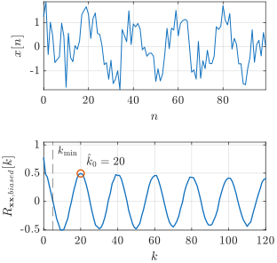
Why the biased ACF The biased form is preferred because the unbiased ACF \(R_{\bxx ,unbiased}[k]\) divides by \(L-k\) (Eq. (21.18)) and so inflates the variance for large \(k\), producing spurious peaks near the tail. The biased ACF uses the constant denominator \(L\), trading a small downward bias for a much better-behaved peak search.
ACF-peak vs. periodogram-peak
The two estimators are Wiener-Khinchin duals: peaks of \(S_{\bxx }[k]\) and peaks of \(R_{\bxx }[k]\) encode the same periodicity, sampled on the frequency axis or the lag axis respectively.
-
• Periodogram-peak (Eq. (20.47)): searches a (possibly zero-padded) frequency grid; high frequency resolution but sensitive to spectral leakage and windowing.
-
• ACF-peak (Eq. (21.39)): integer-lag resolution, \(\Delta F \approx F_s/\hat {k}_0^2\), coarse for small \(\hat {k}_0\) (high frequencies) and fine for large \(\hat {k}_0\) (low frequencies).
-
Example 21.3: A signal contains only the harmonics \(2F_0\), \(3F_0\) and \(4F_0\) of \(F_0=50\) Hz, with amplitudes decaying in that order; the fundamental itself is absent. Its periodogram, the top panel of Fig. 21.5, has lines at \(100\), \(150\) and \(200\) Hz and nothing at \(50\) Hz, so a periodogram-peak search returns the strongest line, \(100\) Hz, which is twice the true value.
The sum of the harmonics is nevertheless periodic with period \(1/F_0\), since \(50\) Hz is the greatest common divisor of the three frequencies. Its biased ACF, the bottom panel, therefore peaks at \(\hat {k}_0=20\) and returns the correct \(\hat {F}_0=50\) Hz.
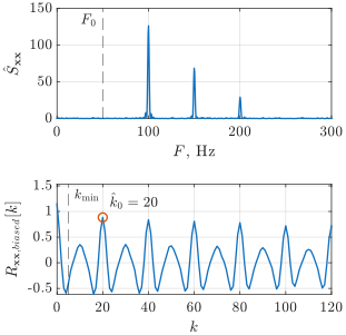
This is the missing fundamental case, and it is why the autocorrelation method is the canonical pitch-detection approach in speech and audio processing, where the fundamental period is read off as \(\hat {k}_0\). Selecting a peak in the frequency domain instead risks returning a harmonic, an error of a whole octave for the \(2F_0\) line.
Tip:
-
• Sub-sample lag refinement: fit a parabola to \(R_{\bxx ,biased}[\hat {k}_0-1],R_{\bxx ,biased}[\hat {k}_0],R_{\bxx ,biased}[\hat {k}_0+1]\) and use its analytic vertex as a fractional-lag estimate, analogous to parabolic peak of the periodogram in (20.48).
21.3 AR(p) Model
The auto-regressive (AR) signal model describes a signal \(y[n]\) as a linear combination of its \(p\) previous samples plus noise. Formally, an \(AR(p)\) model is
\(\seteqnumber{0}{}{40}\)\begin{equation} \begin{aligned} y[n] &=h_1y[n-1] + h_2y[n-2] + \cdots + h_{p}y[n-p] + \epsilon [n]\\ &=\sum _{m=1}^p h_my[n-m]+ \epsilon [n] \end {aligned} \end{equation}
and the prediction is of the form
\(\seteqnumber{0}{}{41}\)\begin{equation} \hat {y}[n] =\sum _{m=1}^p h_my[n-m] \end{equation}
where \(h_1, \ldots ,h_p\) are the AR model coefficients and \(p\) is the model order that is chosen as hyper-parameter.
This model can be easily formulated in the matrix form by using \(L\) sample of \(y[n]\), by
\(\seteqnumber{0}{}{42}\)\begin{equation} \label {eq:ar_prediction} \hat {\by }= \begin{bmatrix} \hat {y}[1] \\ \hat {y}[2]\\ \vdots \\ \hat {y}[L-2] \\ \hat {y}[L-1] \end {bmatrix},\; \bX =\begin{bmatrix} y[0] & 0 & \cdots & 0\\ y[1] & y[0] & \cdots & 0 \\ \vdots & \vdots & \ddots & \vdots \\ y[L-3] & y[L-4] & \cdots & y[L-p-2]\\ y[L-2] & y[L-3] & \cdots & y[L-p-1]\\ \end {bmatrix},\; \bh =\begin{bmatrix} h_1 \\ h_2 \\ \vdots \\ h_{p} \end {bmatrix} \end{equation}
where the corresponding dimensions are \(\hat {\by }\in \Re ^{L-1},\bX \in \Re ^{L-1\times p},\bh \in \Re ^p\).
The AR coefficients \(\bh \) can be found by a LS regression that minimizes the MSE loss
\(\seteqnumber{0}{}{43}\)\begin{equation} \mathcal {L}(h_i) = \sum _n \left (y[n]-\hat {y}[n]\right )^2 = \norm {\by -\bX \bh }^2. \end{equation}
The LS solution is straightforward,
\(\seteqnumber{0}{}{44}\)\begin{equation} \label {eq:normal_eq_matrix} \bh = {\left (\bX ^T\bX \right )^{-1}}\bX ^T\by . \end{equation}
Note, the general approach for evaluation of \(\bh \) is presented in the following section.
-
Example 21.4: Learn linear prediction of \(y[8]\) for \(p=3\) and signal \(y[0],y[1],\ldots ,y[7]\).
-
\(\seteqnumber{0}{}{45}\)
\begin{equation} \bX =\begin{bmatrix} y[0] & 0 & 0 \\ y[1] & y[0] & 0 \\ y[2] & y[1] & y[0] \\ y[3] & y[2] & y[1] \\ y[4] & y[3] & y[2] \\ y[5] & y[4] & y[3] \\ y[6] & y[5] & y[4] \end {bmatrix},\; \bh =\begin{bmatrix} h_1 \\ h_2 \\ h_3 \end {bmatrix}\; \by = \begin{bmatrix} y[1] \\ y[2] \\ y[3]\\ y[4]\\ y[5] \\y[6] \\ y[7] \end {bmatrix} \end{equation}
Finding vector \(\bh \) values is (almost) trivial by a minimum of the loss function of the form
\(\seteqnumber{0}{}{46}\)\begin{equation} \loss = \norm {\by -\bX \bh }^2. \end{equation}
Once found, \(\hat {y}[8] = h_1y[7] + h_2y[6] + h_3y[5]\).
-
\(\seteqnumber{0}{}{45}\)
21.3.1 Yule-Walker Form
The resulting \(\bX ^T\bX \) matrix is termed (Toeplitz) auto-correlation matrix and can be interpreted in terms of auto-correlation values,
\(\seteqnumber{0}{}{47}\)\begin{equation} \begin{aligned} \bR &= \bX ^T\bX \\ &= \begin{bmatrix} R_{\by \by }[0] & R_{\by \by }[1] & \cdots & R_{\by \by }[p-1]\\ R_{\by \by }[1] & R_{\by \by }[0] & \cdots & R_{\by \by }[p-2]\\ \vdots & \vdots & \ddots & \vdots \\ R_{\by \by }[p-1] & R_{\by \by }[p-2] & \cdots & R_{\by \by }[0] \end {bmatrix}, \end {aligned} \end{equation}
where unscaled (or biased) \(R_{\by \by }[k]\) is defined above. It is common practice to ignore the changes in the vector lengths in calculating (biased) ACF for the same time-shift for \(p\ll L\), e.g. diagonal matrix values are
\(\seteqnumber{0}{}{48}\)\begin{equation} R_\byy [0] = \sum _{n=0}^{L-1}y^2[n] \approx \sum _{n=0}^{L-\textbf {2}}y^2[n] \end{equation}
The vector \(\bX ^T\by \) is also comprised of the corresponding \(R_{\byy }[k]\) values,
\(\seteqnumber{0}{}{49}\)\begin{equation} \br = \bX ^T\by = \begin{bmatrix} R_\byy [1]\\ R_\byy [2]\\ \vdots \\ R_\byy [p]\\ \end {bmatrix} \end{equation}
Using these formulations, the resulting coefficients are given by a solution of a set of linear equations,
\(\seteqnumber{0}{}{50}\)\begin{equation} \bR \bh = \br \end{equation}
and the result is similar to Eq. (21.45),
\(\seteqnumber{0}{}{51}\)\begin{equation} \bh = \bR ^{-1}\br \end{equation}
The use of a \(R_{\bx \bx ,biased}[k]\) (biased ACF, Eq. (21.14)) guaranties the numerically stable solution [15, Theorem 6.1].
Squared error The resulting loss (squared error) is given by (following Eqs. (3.21) and (21.33))
\(\seteqnumber{0}{}{52}\)\begin{equation} \begin{aligned} \loss _{min} &= R_\bxx [0] - \sum _{k=1}^p h_kR_\bxx [k] \end {aligned} \end{equation}
Theoretically, higher value of \(p\) results in lower loss in the presence of the sufficiently long correlation time (Eq. (21.21)). Note, the accuracy drops for high values of \(p\) to due to reduced accuracy of \(R_\bxx [p]\).
-
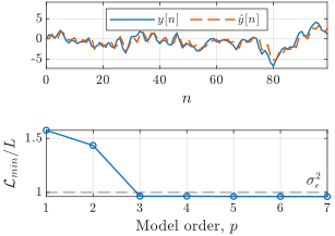
Example 21.5: A synthetic AR(3) signal of length \(L=1000\) is generated by driving the model with white noise of variance \(\sigma _\epsilon ^2=1\) and the true coefficients \(\bh =(1.2,-0.9,0.6)\).
Solving Eq. (21.45) at the correct order, \(p=3\), returns \(\hat {\bh }=(1.19,-0.88,0.57)\), within a few percent of the true values, and the resulting one-step prediction follows the signal closely (top panel of Fig. 21.6).
Repeating the fit for \(p=1,\ldots ,7\) gives the MSE, \(\loss _{min}/L\), of the bottom panel. It falls steeply while \(p\) is below the true order, from \(1.57\) at \(p=1\) to \(0.96\) at \(p=3\), and is flat afterwards, so the elbow of the curve marks the model order.
The flat part sits at \(\approx \sigma _\epsilon ^2\), the variance of the driving noise. Once every predictable component is captured, the residual is the noise itself, and no additional coefficient can lower the loss below it. The coefficients returned for \(p>3\) are indeed close to zero, and their estimates rely on \(R_\byy [k]\) at the largest lags, where the accuracy is lowest.
The commonly adopted notation of the signal model in most of the books and software packages is
\(\seteqnumber{0}{}{53}\)\begin{equation} \sum _{m=0}^p a_m y[n-m] = \epsilon [n] \end{equation}
with \(a_0 = 1\) and \(a_m = - h_m\).
This definition follows discrete-time definition and the corresponding Z-transform of all-pole system. It also can be directly applied as a denominator coefficients for filter command.
Biased signal The presence of a non-zero average (bias) in the signal modifies the AR model formulation. Instead of assuming a zero-mean process, a constant bias term \(\mu \) is introduced,
\(\seteqnumber{0}{}{54}\)\begin{equation} \label {eq:ar_biased} \begin{aligned} \hat {y}[n] &=\mu + h_1y[n-1] + h_2y[n-2] + \cdots + h_{p}y[n-p] + \epsilon [n] \end {aligned} \end{equation}
In matrix form, this requires adding a column of ones \(\bOne _M\) to the data matrix \(\bX \), similarly to how it is done in multivariate LS (Eq.(3.7)).
Tips:
-
• For computational and memory efficiency, the Levinson-Durbin algorithm \(O\left (L^2\right )\) is often used to solve for AR coefficients 1, instead of direct \(O\left (L^3\right )\).
-
• The AR parameters \(\bh \) are also referred to as linear prediction coefficients (LPC), emphasizing their role in predicting the current value from past samples.
-
• The auto-correlation matrix \(\bR \) is guaranteed to be positive-definite (and, therefore, invertible) for ordinary or biased definitions (normalization constants reduce each other in (21.45)).
-
• Theoretically, the AR model coefficients can be regularized to prevent overfitting.
-
• Although this section focuses on linear AR models, nonlinear variants also exist, allowing modeling of more complex dynamics.
-
• Note, there are other methods for LPC calculation, such as Burg’s method, as it is done in librosa.lpc.
1 For example, solve_toeplitz
21.3.2 Moving Average Filter
A simple special case of an AR-like model is the moving average filter, where all coefficients are equal and sum to one, \(h_i=\dfrac {1}{p}\). In this case,
\(\seteqnumber{0}{}{55}\)\begin{equation} \label {eq-moving-average} \begin{aligned} \hat {y}[n] &= \frac {1}{p}\left (y[n-1] + \cdots + y[n-p]\right )\\ &=\frac {1}{p}\sum _{m=1}^p y[n-m] \end {aligned} \end{equation}
This is not strictly an AR model but shares the idea of using past samples. It smooths the signal by averaging the most recent \(p\) values.
21.3.3 Nearest Neighbor (Naïve)
A simple baseline is to use the immediate past sample as the prediction with \(h_1=1\),
\(\seteqnumber{0}{}{56}\)\begin{equation} \label {eq-ts-1nn} \hat {y}[n] = y[n-1] \end{equation}
This "1-nearest neighbor" approach ignores signal dynamics and history. While often not very accurate, it serves as a useful baseline to compare against more sophisticated models.
-
Example 21.6 (Naive baseline vs. AR(1)): The naive predictor differs from the AR(1) model of Eq. (21.1) in one respect only: it forces \(h_1=1\) instead of fitting it. The cost of that shortcut follows from the ACF. Its error power is
\(\seteqnumber{0}{}{57}\)\begin{equation} \sum _n\left (x[n]-x[n-1]\right )^2 = 2\left (R_\bxx [0]-R_\bxx [1]\right ) = 2R_\bxx [0]\left (1-R_{\bxx ,norm}[1]\right ), \end{equation}
while the fitted coefficient attains \(\loss _{min}(h_1)=R_\bxx [0]\left (1-R^2_{\bxx ,norm}[1]\right )\) by Eq. (21.33). Writing \(h_1\approx R_{\bxx ,norm}[1]\), their ratio is
\(\seteqnumber{0}{}{58}\)\begin{equation} \label {eq-naive-penalty} \frac {\MSE _{naive}}{\MSE _{min}} = \frac {2\left (1-h_1\right )}{1-h_1^2} = \frac {2}{1+h_1}. \end{equation}
The penalty is therefore governed by \(h_1\) alone, Fig. 21.7. For \(h_1\to 1\) the ratio tends to \(1\) and the naive predictor is as good as the fitted one. For \(h_1=0.5\) it costs \(4/3\) in MSE, some \(15\%\) in RMSE, and for a white signal, \(h_1=0\), it doubles the error power, whereas the best one-coefficient prediction is \(\hat {x}[n]=0\). For \(h_1<0\), that is a signal alternating in sign, it is worse still.
For the record of Fig. 21.1, with \(h_1=0.9577\), the fitted predictor reaches \(\RMSE =0.999\) and the naive one \(\RMSE =1.010\), a gap of \(1.1\%\), as predicted by Eq. (21.59).
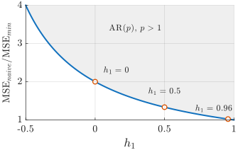
A strongly correlated signal makes the naive predictor hard to beat: at \(h_1\approx 0.96\) it is within about \(1\%\) of the best achievable one-coefficient prediction. Reporting that a model beats the naive baseline by such a margin demonstrates almost nothing about the model.
21.4 Linear Prediction of Sinusoidal Signal
Consider the noise-free sinusoidal signal
\(\seteqnumber{0}{}{59}\)\begin{equation} y[n] = \cos (\omega _0 n) \end{equation}
For simplicity, phase is initially taken as zero. We aim to model it with
\(\seteqnumber{0}{}{60}\)\begin{equation} \hat {y}[n+1] = h_0y[n] +h_1y[n-1] \end{equation}
The corresponding loss is
\(\seteqnumber{0}{}{61}\)\begin{equation} \begin{aligned} \loss (h_0,h_1) &= \sum _n \left (y[n+1]-\hat {y}[n+1]\right )^2\\ &= \sum _n \left (y[n+1]-h_0y[n]-h_1y[n-1]\right )^2\\ \end {aligned} \end{equation}
The required minimum is given by a solution of a system of normal equations,
\(\seteqnumber{0}{}{62}\)\begin{equation} \begin{cases} \dfrac {\partial }{\partial h_0} \loss (h_0,h_1) = 0\\[9pt] \dfrac {\partial }{\partial h_1} \loss (h_0,h_1) = 0\\ \end {cases} \end{equation}
The resulting equations are
\(\seteqnumber{0}{}{63}\)\begin{equation} \begin{cases} \displaystyle 2\sum _n \left (y[n+1] - h_0y[n] - h_1y[n-1]\right )\cdot (-y[n]) = 0\\[16pt] \displaystyle 2\sum _n \left (y[n+1] - h_0y[n] - h_1y[n-1]\right )\cdot (-y[n-1]) = 0\\ \end {cases} \end{equation}
These equations involve sums of trigonometrical functions. Using standard trigonometric identities and assuming a large number of samples \(L\), these sums simplify due to the oscillatory nature of sine and cosine functions.
Some important quantities are
\(\seteqnumber{0}{}{64}\)\begin{equation} \begin{aligned} y[n+1]y[n] &=\cos (\omega _0[n])\cos (\omega _0[n+1])\\ &=\cos (\omega _0n)\left [\cos (\omega _0)\cos (\omega _0 n)-\sin (\omega _0)\sin (\omega _0 n)\right ]\\ &=\cos (\omega _0)\cos [2](\omega _0n)-\sin (\omega _0)\cos (\omega _0n)\sin (\omega _0n) \end {aligned} \end{equation}
For \(1/\omega _0\ll L\), the common assumption is
\(\seteqnumber{0}{}{65}\)\begin{align*} \sum _n \cos [2](\omega _0n) &\approx \frac {L}{2}\\ \sum _n \cos (\omega _0n)\sin (\omega _0n) &\approx 0\\ \sum _n y[n+1]y[n] &\approx \frac {L}{2}\cos (\omega _0)\\ &\approx \sum _n y[n]y[n-1]\\ \sum _n y^2[n] &=\sum _n \cos [2](\omega _0n)\\ &\approx \sum _n y^2[n-1] \approx \frac {L}{2}\\ \sum _n y[n+1]y[n-1] &=\frac {1}{2}\sum _n \cos (2\omega _0n) + \frac {1}{2}\sum _n \cos (2\omega _0) \\ &\approx \frac {L}{2}\cos (2\omega _0) \end{align*} The approximations show that sum terms reduce to manageable forms. Substituting these approximations into the normal equations leads to a system
\(\seteqnumber{0}{}{65}\)\begin{equation} \begin{aligned} h_0\frac {L}{2} &+ h_1\frac {L}{2}\cos (\omega _0) &&= \frac {L}{2}\cos (\omega _0)\\ h_0\frac {L}{2}\cos (\omega _0) &+h_1\frac {L}{2} &&= \frac {L}{2}\cos (2\omega _0) \end {aligned} \end{equation}
Solving these two linear equations for prediction coefficients yields
\(\seteqnumber{0}{}{66}\)\begin{equation} \begin{aligned} h_0 &= 2\cos (\omega _0)\\ h_1 &= -1 \end {aligned} \end{equation}
This result is exact in the idealized scenario of an infinite, noise-free sinusoid.
If the signal had a phase \(\theta \),
\(\seteqnumber{0}{}{67}\)\begin{equation} y[n] = \cos (\omega _0 n+\theta ) \end{equation}
the same coefficients still apply, only the initial conditions (the first two samples) differ,
\(\seteqnumber{0}{}{68}\)\begin{equation} \begin{aligned} y[0] &=\cos (\theta )\\ y[1] &=\cos (\omega _0+\theta ). \end {aligned} \end{equation}
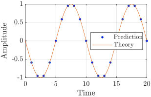
The AR(2) model still perfectly represents the sinusoidal sequence. The example of the resulting signal is presented in Fig. 21.8.
Results interpretation:
-
• Any complex signal can be thought of as a sum of sinusoids. In theory, each sinusoidal component can be perfectly modeled by an AR(2) process corresponding to its frequency.
-
• In practice, signals are finite in length and often corrupted by noise. Under these realistic conditions, perfect prediction is not achievable, and the AR model’s accuracy diminishes as noise and non-idealities increase. The prediction horizon is limited even for a periodic low-noise signals.
-
• Nevertheless, this analysis provides a foundational insight: sinusoids have a natural AR(p) representation, explaining why AR(p) models are often effective in capturing periodic components of signals for a small-step prediction.
21.5 Partial auto-correlation function
-
Goal: The partial autocorrelation function (PACF) measures the correlation between a time series and its lagged values after removing the influence of all shorter lags. In other words, the PACF at lag \(k\) shows the direct effect of \(y[n-k]\) on \(y[n]\), excluding any intermediary correlations through lags less than \(k\).
The partial autocorrelation at \(k\) is the correlation that results after removing the effect of any correlations due to the terms at shorter lags,
\[ \underline {x[0]},\underbrace {x[1],x[2],\ldots ,x[j-1]}_{\text {partial out}},\underline {x[j]},x[j+1],\ldots \]
The PACF at lag \(k\) can be extracted by fitting an AR(k) model and observing the coefficient associated with \(y[n-k]\) in this model2. For each \(k\),
\(\seteqnumber{0}{}{69}\)\begin{equation} \hat {y}_{k}[n] = \phi _{k,1} y[n-1] + \phi _{k,2} y[n-2] + ... + \phi _{k,k} y[n-k] + \epsilon [n] \end{equation}
The \(k\)-th partial autocorrelation, \(\beta [k]\) is \(\phi _{k,k}\), the coefficient of \(y[n-k]\) in the AR(k) model. Each of these AR(k) models can be solved using standard LS methods.
The algorithm is as follows:
-
• For the first value of PACF, \(\beta [1]\), fit AR(1) model
\(\seteqnumber{0}{}{70}\)\begin{equation} \hat {y}_{1}[n] = \phi _{1,1} y[n-1] + \epsilon [n] \end{equation}
and the coefficient \(\beta [1]=\hat {\phi }_{1,1}\) is given by the model solution, \(h_1\) (Eq. (21.5)).
-
• For the second order PACF, it would be the \(\beta [2]=\phi _{2,2}\) coefficient of AR(2) model,
\(\seteqnumber{0}{}{71}\)\begin{equation} \hat {y}_2[n] = \phi _{2,1} y[n-1] + \phi _{2,2} y[n-2] + \epsilon [n] \end{equation}
-
• Continue this process up to the desired lag, each time extracting the coefficient of the highest-order lag as the PACF value.
Tip:
-
• While the ACF reflects both direct and indirect correlations (where an earlier lag may influence a later lag through intermediate values), the PACF isolates the direct contribution of each individual lag once all shorter-term effects are factored out.
-
• Though conceptually the PACF is obtained by fitting multiple AR models, practically more efficient algorithms like the Levinson-Durbin recursion can compute these values quickly and without having to solve a new LS problem at every step.
21.5.1 Relation between PACF and AR(p)
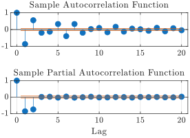
The order \(p\) of AR(p) model is related to the statistically significant (over a confidence bound) coefficients of PACF. Observing where the PACF cuts off helps identify the appropriate order \(p\) for AR(p) model fitting. An example of a synthetic signal analysis with \(p=2\) is presented in Fig. 21.9.
21.6 MA model
Another model is the moving average model (MA), where the output is a linear combination of the noise values at the different times [12, Example 4.3, pp. 90]
\(\seteqnumber{0}{}{72}\)\begin{equation} y[n] = \epsilon [n] + c_1\epsilon [n-1] + \cdots + c_{q}\epsilon [n-q] \end{equation}
Because the noise terms \(\epsilon [n]\) are not directly observable (unlike the past outputs in AR modeling), deriving a closed-form solution for MA parameters through simple linear regression is not as direct and is not presented here. 3 While the underlying theory is well-established, practical estimation of MA parameters often involves advanced numerical methods rather than a simple closed-form solution.
21.6.1 MA and AR relations
There exists a duality between AR and MA processes in terms of infinite expansions:
Presenting AR(p) as MA(\(\infty \)) An AR model can be represented as an infinite MA model when the autoregressive parameters are stable. Consider the recursive simple AR(1),
\(\seteqnumber{0}{}{73}\)\begin{equation} \begin{aligned} y[n] &= h_1y[n-1] + \epsilon [n]\\ &= h_1(h_1y[n-2] + \epsilon [n-1]) + \epsilon [n]\\ &= h_1^2y[n-2] + h_1\epsilon [n-1] + \epsilon [n]\\ &= h_1^3y[n-3] + h_1^2\epsilon [n-2] + h_1\epsilon [n-1] + \epsilon [n] \end {aligned} \end{equation}
Continuing this process indefinitely and assuming stability, \(h_1<1, \lim \limits _{k\rightarrow \infty }h_1^k\rightarrow 0\), we have
\(\seteqnumber{0}{}{74}\)\begin{equation} \begin{aligned} y[n] &= \epsilon [n] + h_1\epsilon [n-1] + h_1^2\epsilon [n-2] + h_1^3\epsilon [n-3] + \cdots \\ &=\sum _{i=0}^\infty h_1^i\epsilon [n-i] \end {aligned} \end{equation}
that it is MA(\(\infty \)) model, where the coefficients of the MA representation are the infinite geometric sequence powers of \(h_1\).
Presenting MA(1) as AR(\(\infty \)) An MA(1) process is given by
\(\seteqnumber{0}{}{75}\)\begin{equation} x[n] = \epsilon [n] + c_1\,\epsilon [n-1]. \end{equation}
We can express the process as an infinite-order AR\((\infty )\) model.
First, note that we can write
\(\seteqnumber{0}{}{76}\)\begin{align*} \epsilon [n] &= x[n] - c_1\,\epsilon [n-1].\\ \epsilon [n-1] &= x[n-1] - c_1\,\epsilon [n-2]\\ \epsilon [n-2] &= x[n-2] - c_1\,\epsilon [n-3] \end{align*} and so on. Substituting for \(\epsilon [n-i]\) recursively, we have
\(\seteqnumber{0}{}{76}\)\begin{equation} \begin{aligned} \epsilon [n] &= x[n] - c_1\left (x[n-1] - c_1\,\epsilon [n-2]\right )\\[1mm] &= x[n] - c_1\,x[n-1] + c_1^2\,\epsilon [n-2]\\[1mm] &= x[n] - c_1\,x[n-1] + c_1^2\left (x[n-2] - c_1\,\epsilon [n-3]\right )\\[1mm] &= x[n] - c_1\,x[n-1] + c_1^2\,x[n-2] - c_1^3\,\epsilon [n-3]\\[1mm] &\,\,\,\vdots \\[1mm] &= \sum _{i=0}^\infty (-c_1)^i\,x[n-i]. \end {aligned} \end{equation}
Rearranging, the AR\((\infty )\) representation becomes
\(\seteqnumber{0}{}{77}\)\begin{equation} x[n] = \epsilon [n] + \sum _{i=1}^\infty (-c_1)^i\,x[n-i]. \end{equation}
Note the invertibility condition, \(|c_1| < 1\).
Interpretation AR and MA are not mutually exclusive categories. A stable AR process can be seen as a special case of an infinite MA, and a stable MA can be thought of as an infinite AR.
21.6.2 The relation between MA(q) and ACF
The MA(q) model has a distinctive fingerprint in terms of its ACF; it is nonzero for up to lag \(q\) and essentially zero afterward (except for sampling and noise effects). Just as the partial autocorrelation function (PACF) helps determine the order \(p\) of an AR(p) process by pinpointing where its PACF cuts off (Sec. 21.5.1), the ACF helps identify the order \(q\) of an MA(q) process.
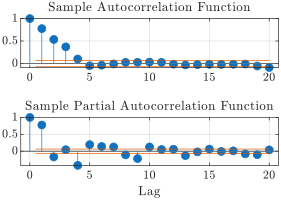
An example of a synthetic MA(4) signal analysis is presented in Fig. 21.10. After lag 4, the ACF values remain within the confidence bounds, essentially zero, suggesting the data arise from an MA(4) process.
21.7 ARMA
The ARMA(p,q) model is given by
\(\seteqnumber{0}{}{78}\)\begin{equation} \begin{aligned} \hat {y}[n] &= h_1y[n-1] + \cdots + h_py[n-p] \\ &+ c_1\epsilon [n-1] + \cdots + c_q\epsilon [n-q] + \epsilon [n]\\ &=\sum _{i=1}^{p}h_iy[n-i] + \sum _{k=0}^qc_k\epsilon [n-k] \end {aligned}, \end{equation}
where \(c_0=1\) by definition.
One of the ways to describe MA part of ARMA, is that MA uses to model the difference unexplained by AR model,
\(\seteqnumber{0}{}{79}\)\begin{equation} \hat {y}[n] - \sum _{i=1}^{p}h_iy[n-i] = \sum _{k=0}^qc_k\epsilon [n-k] \end{equation}
Innovation
The innovation of a signal is the part of the current sample that the signal’s own past cannot predict, that is, the error of the best linear one-step prediction of \(y[n]\) from \(y[n-1],y[n-2],\ldots \) Everything predictable has been taken out of it, so it is white, which is what makes it the natural driving noise of a model of that signal.
Its variance is the floor of the loss. It is what remains once every coefficient has done its work, and no choice of orders reaches below it. The driving noise of a model is thus the innovation of the signal the model generates, and a signal carrying more than one noise source has an innovation that is none of them separately, as the following example shows.
The MA part is not merely a modeling convenience. The following example shows a routine measurement setup in which it appears by itself, with no choice involved.
-
Example 21.7: An AR(1) signal is recorded by a noisy sensor. The hidden state follows
\(\seteqnumber{0}{}{80}\)\begin{equation} \label {eq:arma-sensor-state} y[n] = h_1y[n-1] + \epsilon [n],\quad \abs {h_1}<1, \end{equation}
and the sensor adds a white measurement noise \(v[n]\) of variance \(\sigma _v^2\), independent of the driving noise \(\epsilon [n]\),
\(\seteqnumber{0}{}{81}\)\begin{equation} \label {eq:arma-sensor-obs} z[n] = y[n] + v[n]. \end{equation}
Show that \(z[n]\) is an ARMA(1,1) process. The ACF values below are the per-sample averaged form of Eq. (21.14).
-
Solution: Apply the AR(1) difference of Eq. (21.81) to the observed signal and substitute Eq. (21.82),
\(\seteqnumber{0}{}{82}\)\begin{equation} \label {eq:arma-sensor-u} u[n] \triangleq z[n] - h_1z[n-1] = \epsilon [n] + v[n] - h_1v[n-1], \end{equation}
using \(y[n]-h_1y[n-1]=\epsilon [n]\). The ACF of \(u[n]\) is the per-sample average of the product \(u[n]u[n-k]\). Both noises are white, zero-mean and mutually independent, so such a product averages to zero unless it is the square of one and the same noise sample. At lag \(0\) the three squares \(\epsilon ^2[n]\), \(v^2[n]\) and \(h_1^2v^2[n-1]\) survive. At lag \(1\) the two factors share the single sample \(v[n-1]\), which enters \(u[n]\) as \(-h_1v[n-1]\) and \(u[n-1]\) as \(v[n-1]\). At \(\abs {k}\ge 2\) they share no sample at all, since \(u[n]\) carries only the times \(n\) and \(n-1\). Hence
\(\seteqnumber{0}{}{83}\)\begin{equation} \label {eq:arma-sensor-Ruu} \begin{aligned} R_{\bu \bu }[0] &= \frac {1}{L}\sum _n u^2[n] = \sigma _\epsilon ^2 + \sigma _v^2\left (1+h_1^2\right )\\ R_{\bu \bu }[1] &= \frac {1}{L}\sum _n u[n]u[n-1] = -h_1\sigma _v^2\\ R_{\bu \bu }[k] &= 0,\quad \abs {k}\ge 2. \end {aligned} \end{equation}
An ACF vanishing beyond lag \(1\) is exactly the MA(1) fingerprint of Sec. 21.6.2. The reverse reading is the one used here, and it holds because the MA(1) family is rich enough to match Eq. (21.84): it has two free parameters, \(c_1\) and \(\sigma _\eta ^2\), and its ACF has exactly two free values, at lags \(0\) and \(1\), with all higher lags zero, which is the shape found above. The representation is thus
\(\seteqnumber{0}{}{84}\)\begin{equation} u[n] = \eta [n] + c_1\eta [n-1], \end{equation}
where \(\eta [n]\) is white of variance \(\sigma _\eta ^2\). It is neither \(\epsilon [n]\) nor \(v[n]\), but the innovation of the observed signal, and the equality is one of second-order statistics.
The ACF of the representation follows by the argument used for Eq. (21.84): at lag \(0\) the squares \(\eta ^2[n]\) and \(c_1^2\eta ^2[n-1]\) survive, and at lag \(1\) only the sample \(\eta [n-1]\) shared by the two factors, entering them as \(c_1\eta [n-1]\) and as \(\eta [n-1]\),
\(\seteqnumber{0}{}{85}\)\begin{equation} R_{\bu \bu }[0] = \sigma _\eta ^2\left (1+c_1^2\right ),\qquad R_{\bu \bu }[1] = \sigma _\eta ^2c_1. \end{equation}
These are two equations in the two unknowns, and their ratio cancels \(\sigma _\eta ^2\) and leaves a single equation in \(c_1\),
\(\seteqnumber{0}{}{86}\)\begin{equation} \frac {c_1}{1+c_1^2} = \rho _{\bu \bu }[1] \triangleq \frac {R_{\bu \bu }[1]}{R_{\bu \bu }[0]}, \end{equation}
the lag-\(1\) correlation coefficient of Eq. (21.24). Of the two roots of this quadratic, the invertible one, \(\abs {c_1}<1\), gives
\(\seteqnumber{0}{}{87}\)\begin{equation} \label {eq:arma-sensor-c1} c_1 = \frac {1-\sqrt {1-4\rho _{\bu \bu }^2[1]}}{2\rho _{\bu \bu }[1]},\qquad \sigma _\eta ^2 = \frac {R_{\bu \bu }[1]}{c_1}. \end{equation}
The root is real for any sensor. As \(c_1\) runs over \([-1,1]\), the ratio \(c_1/(1+c_1^2)\) runs over \([-1/2,1/2]\), and Eq. (21.84) keeps the correlation inside that range,
\(\seteqnumber{0}{}{88}\)\begin{equation} \abs {\rho _{\bu \bu }[1]} = \frac {\abs {h_1}\sigma _v^2}{\sigma _\epsilon ^2+\sigma _v^2\left (1+h_1^2\right )} \le \frac {\abs {h_1}}{1+h_1^2} \le \frac {1}{2}. \end{equation}
Substituting back into Eq. (21.83),
\(\seteqnumber{0}{}{89}\)\begin{equation} \label {eq:arma-sensor-result} z[n] = h_1z[n-1] + \eta [n] + c_1\eta [n-1], \end{equation}
which is an ARMA(1,1) model.
-
Three readings of Eq. (21.90) are worth noting.
-
• The AR coefficient survives untouched. The sensor does not change the dynamics of the state, it only contributes the MA term, whose coefficient \(c_1\) carries the sign opposite to \(h_1\).
-
• The limits behave as they should. For \(\sigma _v^2\to 0\) the correlation \(\rho _{\bu \bu }[1]\to 0\) and \(c_1\to 0\), recovering the AR(1) of Eq. (21.81). For \(\sigma _v^2\to \infty \) the correlation tends to \(-h_1/(1+h_1^2)\) and \(c_1\to -h_1\), so the AR and MA parts cancel and \(z[n]\) is white, as expected when the record is all sensor noise.
-
• The order of the MA part counts the noisy measurements, not the states. One noisy sensor adds one MA coefficient.
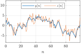
One realization of this setup, with \(h_1=0.9\), \(\sigma _\epsilon ^2=1\) and \(\sigma _v^2=2\), is shown in Fig. 21.11. The sensor noise adds a fast jitter on top of the slow swings of the hidden state, and only the jittered record is available to the model. Its AR(1) difference \(u[n]=z[n]-h_1z[n-1]\) measured on the same record follows Eq. (21.84): the estimated correlation coefficient is \(\hat {\rho }_{\bu \bu }[1]=-0.398\) against the predicted \(-0.390\), and beyond lag \(1\) it scatters about zero, never exceeding \(0.042\) in absolute value. This is the MA(1) fingerprint of Sec. 21.6.2, and it is what makes the MA term of Eq. (21.90) necessary.
Measurement noise attenuates AR coefficients
Fitting an AR(1) model to \(z[n]\) instead of the ARMA(1,1) of Eq. (21.90) returns, by Eq. (21.11),
\(\seteqnumber{0}{}{90}\)\begin{equation} \label {eq:arma-attenuation} \hat {h}_1 = \frac {R_{\bz \bz }[1]}{R_{\bz \bz }[0]} = \frac {\sigma _y^2h_1}{\sigma _y^2+\sigma _v^2} < h_1, \qquad \sigma _y^2=\frac {\sigma _\epsilon ^2}{1-h_1^2}, \end{equation}
because the measurement noise inflates the lag-\(0\) term without touching the lag-\(1\) one. For \(h_1=0.9\), \(\sigma _\epsilon ^2=1\) and \(\sigma _v^2=2\) this gives \(\hat {h}_1=0.65\) against the true \(0.9\): the process looks considerably less predictable than it is. The attenuation grows with the sensor noise and is not cured by a longer record. Adding the MA term is what restores the correct dynamics.
As with AR models (Eq. (21.55)), a constant bias \(\mu \) can be included,
\(\seteqnumber{0}{}{91}\)\begin{equation} \hat {y}[n] =\sum _{i=1}^{p}h_iy[n-i] + \sum _{k=0}^qc_k\epsilon [n-k] + \mu \end{equation}
21.7.1 Order Selection
Both \(p\) and \(q\) are hyper-parameters. They are fixed by fitting a grid of candidate pairs and comparing the resulting losses.
-
Example 21.8: A hidden AR(1) state with \(h_1=0.9\) and driving noise of variance \(\sigma _\epsilon ^2=1\) is read by a sensor adding white noise of variance \(\sigma _v^2=2\), and \(L=2000\) samples of the observation \(z[n]\) are kept after the transient. This is the setup of Example 21.7, so the true order is known: \(z[n]\) is ARMA(1,1) with \(c_1=-0.479\) and an innovation variance \(\sigma _\eta ^2=3.76\), by Eq. (21.88).
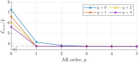
Every pair \((p,q)\) with \(p=0,\ldots ,5\) and \(q=0,\ldots ,3\) is fitted. All fits share same sample set, so that the losses are comparable, and the grid is averaged over \(200\) realizations. The results are given in Table 21.2 and Fig. 21.12, and read as follows.
-
• An MA coefficient buys more than an AR one. At \(p=1\) the loss drops from \(4.151\) to \(3.742\) with the first MA coefficient, while the pure AR route needs \(p=3\) to come within \(1\%\) of that value. This is the finite-sample face of the MA(1) to AR(\(\infty \)) expansion: an MA term can always be traded for AR terms, but only at the price of extra order, and here two coefficients do the work of three.
-
• The loss floor is the innovation variance of the observed signal. It is \(\sigma _\eta ^2=3.76\), and not the \(\sigma _\epsilon ^2=1\) of the hidden state, because the measurement noise is not predictable from the past and no model order can remove it. The plateau of the grid sits on it, the \((1,1)\) entry being \(3.742\). The opposite corner reads the same way: a model of no order predicts nothing, so the \((0,0)\) entry \(7.279\) is the power of the observation itself, \(\sigma _z^2=\sigma _\epsilon ^2/(1-h_1^2)+\sigma _v^2=7.263\).
-
• The plateau, not the minimum, marks the order. The loss never increases with \(p\) or \(q\), so the smallest entry is always the bottom-right corner, \((5,3)\) here. What the grid does show is where the surface goes flat, and the order to report is the cheapest one reaching that plateau, \((p,q)=(1,1)\), the true order of \(z[n]\).
-
| AR order, \(p\) | \(q=0\) | \(q=1\) | \(q=2\) | \(q=3\) |
| \(0\) | \(7.279\) | \(6.619\) | \(6.082\) | \(5.637\) |
| \(1\) | \(4.151\) | \(\underline {3.742}\) | \(3.740\) | \(3.738\) |
| \(2\) | \(3.820\) | \(3.739\) | \(3.732\) | \(3.730\) |
| \(3\) | \(3.749\) | \(3.735\) | \(3.730\) | \(3.727\) |
| \(4\) | \(3.734\) | \(3.730\) | \(3.728\) | \(3.725\) |
| \(5\) | \(3.728\) | \(3.726\) | \(3.725\) | \(3.723\) |
Tips:
-
• The ACF and PACF fingerprints used for the pure models (Sec. 21.5.1 and Sec. 21.6.2) do not identify an ARMA model. Both of its tails decay without cutting off, so neither plot marks an order, and the two-dimensional search of Table 21.2 is used instead.
-
• Fitting the largest \((p,q)\) affordable is never penalized by the in-sample loss. Comparing models of different order calls for a criterion that charges for parameters, or for a held-out record.
21.7.2 Prediction Horizon
Every fit so far was compared one step ahead. A prediction \(\ell \) steps ahead uses \(y[n],y[n-1],\ldots \) and nothing later, so the model is iterated forward one sample at a time,
\(\seteqnumber{0}{}{93}\)\begin{equation} \label {eq:arma-horizon-rule} \hat {y}[m] = \sum _{i=1}^{p}h_i\hat {y}[m-i] + \sum _{k=1}^{q}c_k\hat {\epsilon }[m-k], \qquad m=n+1,\ldots ,n+\ell , \end{equation}
where the terms of the two sums are
\(\seteqnumber{0}{}{94}\)\begin{equation} \label {eq:arma-horizon-sub} \hat {y}[j] = y[j],\quad j\le n \qquad \qquad \hat {\epsilon }[j] = \begin{cases} \epsilon [j], & j\le n\\ 0, & j>n \end {cases} \end{equation}
A sample past the origin \(n\) has not been observed, so the model uses its own forecast of it, supplied by the recursion itself. An innovation past the origin is white and independent of the record, so its best estimate is \(0\). These two rules are the whole of multi-step prediction, and reading them per model class is what separates the classes.
-
• MA(\(q\)) forgets after \(q\) steps. Its sum has no \(\hat {y}\) terms at all, and once \(\ell >q\) every index \(m-k\) is past the origin, so every term is zeroed and the forecast is the process mean. Its memory is \(q\) samples, no fit can extend it, and beyond that its error is the full power \(\sigma _y^2\) of the signal.
-
• AR(\(p\)) decays but never stops. The recursion feeds on its own output, so a forecast exists at every horizon. It decays with the poles of the model, geometrically as \(h_1^\ell \) for AR(1), and the error climbs toward \(\sigma _y^2\) gradually rather than reaching it at a fixed lag.
-
• ARMA(\(p,q\)) uses both. The MA part corrects the first \(q\) steps and the AR recursion carries everything after that. Its price is that Eq. (21.94) needs \(\epsilon [j]\) for \(j\le n\), which the record does not hold: the innovations are reconstructed by the AR(\(\infty \)) expansion of Sec. 21.6.1, the first stage of the two-stage fit.
-
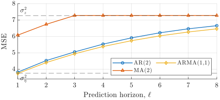
Example 21.9: The noisy-sensor record of Example 21.7 is predicted at horizons \(\ell =1,\ldots ,8\) by three models of two coefficients each: AR(2), MA(2) and ARMA(1,1). Eq. (21.94) is applied here to the observation \(z[n]\) and its innovation \(\eta [n]\). The forecast MSE, averaged over \(200\) realizations, is shown in Fig. 21.13.
-
• The MA model stops predicting at \(\ell =3\). Its curve is flat from there on at \(7.280\), the power of the record, against \(\sigma _z^2=7.263\) for the process. This is not a fitting failure but the structure of Eq. (21.94): past lag \(q=2\) there is nothing left to sum. Raising \(q\) moves the wall further out and never removes it.
-
• The models with an AR part keep predicting. AR(2) has a forecast at every horizon, but at the same budget it trails ARMA(1,1) throughout, from \(3.820\) against \(3.743\) at \(\ell =1\) to \(6.659\) against \(6.467\) at \(\ell =8\), the same order price as at one step, where Table 21.2 needs \(p=3\) to reach the ARMA(1,1) loss. Both approach \(\sigma _z^2\) only gradually, the ARMA(1,1) curve following the closed form \(\sigma _\eta ^2\left (1+\sum _{j=1}^{\ell -1}\psi _j^2\right )\) with \(\psi _j=h_1^{j-1}\left (h_1+c_1\right )\), so the horizon over which a model stays below \(\sigma _z^2\) is what its class buys.
-
Tips:
-
• The horizon is chosen by the application, and it decides the model class before any order is fitted: a model with no AR part cannot serve a horizon longer than its own order.
-
• Two models that tie at \(\ell =1\) can still differ at \(\ell =5\), so a model meant to forecast far ahead is compared at the horizon it will serve.
21.7.3 Rational PSD (*)
Written in the \(a_m\) notation of Eq. (21.93), the two coefficient sets define a pair of frequency functions on the DFT grid \(\omega _k=2\pi k/N\),
\(\seteqnumber{0}{}{95}\)\begin{equation} \label {eq:arma-poly} A(\omega _k) = \sum _{m=0}^p a_m\exp (-j\omega _km),\qquad C(\omega _k) = \sum _{m=0}^q c_m\exp (-j\omega _km), \end{equation}
that is, the DTFT of each coefficient sequence. The driving noise is white, so its PSD is flat (Sec. 21.2 and the left column of Fig. 21.3), and the PSD of the ARMA output is
\(\seteqnumber{0}{}{96}\)\begin{equation} \label {eq:arma-psd} S_\byy [k] = \sigma _\epsilon ^2\frac {\abs {C(\omega _k)}^2}{\abs {A(\omega _k)}^2}. \end{equation}
The PSD is thus a ratio of two polynomials, which is what the ARMA coefficients buy in the frequency domain.
-
• The roots of the denominator, contributed by the AR coefficients and termed poles, drive \(S_\byy [k]\) up near their frequency and produce resonance peaks.
-
• The roots of the numerator, contributed by the MA coefficients and termed zeros, drive it down and produce notches.
-
• A root pair of radius \(r\) at normalized frequency \(f_0\) corresponds to the coefficient triple \(\left (1,-2r\cos (2\pi f_0),r^2\right )\). Its angle sets the frequency, and its radius, approaching \(1\), sets how sharp the peak or how deep the notch becomes. A zero of radius exactly \(1\) gives an exact null, but sits on the boundary of the invertibility condition met above.
-
• An AR(\(p\)) model is all-pole, \(C(\omega _k)=1\). It builds peaks directly and reproduces a notch only by spending several poles on it, which is the frequency-domain form of the order trade-off of Table 21.2. Symmetrically, an MA(\(q\)) model is all-zero and cannot produce a sharp resonance.
-
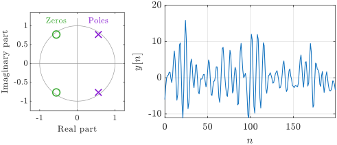
Example 21.10: An ARMA(2,2) model is built from one pole pair of radius \(0.95\) at \(0.15F_s\) and one zero pair of the same radius at \(0.35F_s\), that is
\(\seteqnumber{0}{}{97}\)\begin{equation} \bh = (1.117,\,-0.902),\qquad (c_1,c_2) = (1.117,\,0.902). \end{equation}
The two root pairs are shown in the left panel of Fig. 21.14: both sit at radius \(0.95\), the poles at the angle \(2\pi \cdot 0.15\) and the zeros at \(2\pi \cdot 0.35\). A segment of one realization is drawn in the right panel, where the pole pair is visible as a narrowband oscillation of about \(1/0.15\approx 7\) samples per period.
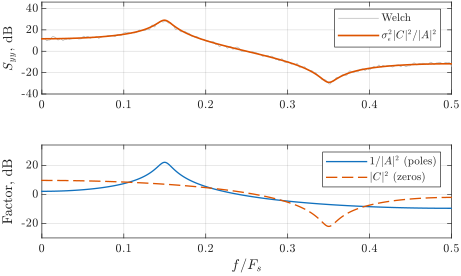
Its PSD, Eq. (21.97), is drawn in the top panel of Fig. 21.15 together with a Welch estimate (Sec. 20.7.4) of one realization, which follows it closely. The peak sits at \(0.15F_s\) and the notch at \(0.35F_s\), exactly at the root frequencies, and they are separated by \(58\) dB.
The bottom panel separates the two factors of Eq. (21.97). The peak comes entirely from \(1/\abs {A(\omega _k)}^2\) and the notch entirely from \(\abs {C(\omega _k)}^2\), each factor being flat where the other acts. Removing the MA part would leave the peak untouched and the notch gone.
This combination is why ARMA is the natural model for signals whose spectra carry both resonances and anti-resonances, whereas an AR model of comparable order captures only the resonances.