Machine Learning & Signals Learning
25 Object Detection
The image notation of Ch. 23 carries over: an input image \(\bX \in \mathbb {R}^{H\times W\times C_{\text {in}}}\), and \(C\) object classes.
Detection sits at the end of a natural progression of image-level tasks, each adding one more degree of output complexity:
-
• Image classification (Ch. 23)
-
– Dataset provides one label per image, \(1\,\text {image}\to 1\,\text {class}\).
-
– Model output is a probability simplex \(\Delta ^{C}\) over the \(C\) classes.
-
-
• Classification with localization (currently not discussed in-depth in this chapter):
-
– Dataset provides one label and one bounding box for a single dominant object, \(1\,\text {image}\to 1\,\text {class}+1\,\text {box}\).
-
– Model output is a probability simplex \(\Delta ^{C}\) and four box coordinates. The output shape is still fixed, so a single regression head bolted onto a classifier suffices.
-
-
• Object detection (this chapter)
-
– Dataset provides a variable-length list of (class, box) annotations per image, \(1\,\text {image}\to N\,(\text {class}+\text {box})\) with \(N\) unknown in advance.
-
– Model output is a set of (class, box, score) tuples, where the score \(s\in [0,1]\) is a per-(box, class) confidence used to rank the prediction against others on the precision-recall curve (Sec. 25.2).
-
– Makes the output variable-length (an image may contain zero, one or many objects).
-
– Couples a regression (box coordinates) and a classification (class + objectness), evaluated jointly.
-
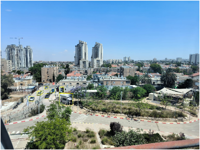
25.1 Bounding-box principle
A bounding box is the smallest axis-aligned rectangle that fully encloses an object in the image plane. Two equivalent four-number parameterizations are used:
-
• Corner form \(b=(x_1,y_1,x_2,y_2)\): top-left and bottom-right pixel coordinates, with \(x_1<x_2\) and \(y_1<y_2\). Convenient for IoU and matching (Sec. 25.2).
-
• Center-size form \(b=(x_c,y_c,w,h)\): box center and width/height, with each coordinate normalized to \([0,1]\) by dividing \(x_c,w\) by the image width and \(y_c,h\) by the image height. Normalization makes the four numbers resolution-independent: the same box parameters describe the object before and after resizing a \(1920\times 1080\) image to the \(640\times 640\) training crop, so one regression target stays valid across the multi-scale training augmentations (Sec. 23.4) and the variable camera resolutions seen at inference. The parameterization also decouples location (\(x_c,y_c\)) from scale (\(w,h\)).
The box carries no orientation (no rotation) and no shape information beyond the rectangle; tighter outlines require instance segmentation (Ch. 24). A box is considered correct, against a ground-truth box of the same class, when their overlap exceeds an IoU threshold (Sec. 25.2). A geometric augmentation moves the boxes together with the image: after a flip, zoom or shift the four numbers are recomputed, and after a rotation the box is redrawn as the smallest axis-aligned rectangle around the rotated corners, which makes it looser than the object.
When to use it Detection is the right tool when you must locate and count multiple objects of possibly overlapping categories in a scene, and a bounding box is precise enough (otherwise use instance segmentation). Counter-indications:
-
• A single dominant object per image \(\to \) classifier (Ch. 23).
-
• Pixel-precise contours required \(\to \) segmentation (Ch. 24).
-
• Open-set identification (who is this person?) \(\to \) Siamese / embedding approach (Ch. 26).
25.2 Performance metrics
An object detector (the model being evaluated) outputs a set of scored boxes per image, and the metric has to collapse that set into a single comparable number. It does so through a four-stage pipeline, each stage feeding the next:
-
1. Match and label: pair each predicted box with a ground-truth box by bounding-box IoU, label it TP or FP, and count the missed ground truths as FN.
-
2. Sweep: vary the confidence cut-off to trace a precision–recall curve.
-
3. Integrate: collapse that curve into one average precision (AP) at a fixed IoU threshold.
-
4. Average: average AP over classes (mAP) and over IoU thresholds (mAP@[.5:.95]).
The subsections below walk these stages in order; non-maximum suppression is an inference-time aside (it reuses the same IoU test) inserted between Stages 1 and 2.
25.2.1 Box matching and TP/FP/FN labeling
Matching is done one class at a time and repeated identically for each class (Stage 4 then averages across classes).
The detector’s class-\(c\) predictions are a set of boxes \(\{\hat b_i\}\) with confidence scores \(\{s_i\}\), which must be scored against the class-\(c\) ground-truth boxes \(\{b_j\}\). Matching turns these two box sets into TP, FP, and FN counts.
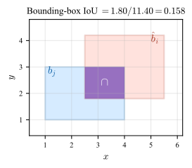
When does a box count as correct? Overlap is measured by the bounding-box IoU (Eq. 24.5, Fig. 25.2): a prediction can match a ground-truth box only if their IoU clears a threshold \(\tau \in [0,1]\) (Pascal VOC uses \(\tau =0.5\); a stricter \(\tau \) demands tighter boxes).
The matching rule Several predictions may overlap the same object, so to keep the count unambiguous they are matched greedily in order of confidence:
-
1. Sort the predictions by descending confidence scores \(\{s_i\}\) and walk down the list.
-
2. Each \(\hat b_i\) claims the still-unclaimed ground-truth box \(b_j\) with which its \(\text {IoU}(\hat b_i, b_j)\ge \tau \) is highest.
This sorts every box into one of three outcomes:
-
• True positive (TP): the claimed box clears \(\text {IoU}(\hat b_i, b_j)\ge \tau \), and that ground truth leaves the pool.
-
• False positive (FP): the prediction wins no valid claim, either because it overlaps no ground truth above \(\tau \) (a misplaced box) or because the ground truth it overlaps was already taken by a higher-scoring prediction (a duplicate detection).
-
• False negative (FN): a ground-truth box left unclaimed once every prediction has been processed.
Why there is no TN This reduces single-image detection to TP, FP, FN counts per class, almost the binary classification setting of Chapter 17. The missing fourth cell is TN: a true negative would be a correctly emitted “no object here” decision, but the negative space is every possible box in the image plane (infinitely many), so TN is undefined and not counted. This is why detection metrics use precision and recall (which need only TP, FP, FN) and never accuracy or specificity (which need TN).
What IoU threshold counts as a good match?
-
• \(\tau =0.5\): the lenient default; tolerates loose boxes and is what Pascal VOC (Sec. 24.3) adopted.
-
• \(\tau =0.75\): strict; requires tight localization.
-
• \(\tau \in \{0.5,0.55,\dots ,0.95\}\): averaging the metric over this range (rather than picking one \(\tau \)) is the COCO (Sec. 24.3) convention.
For a single image, \(\text {IoU}\ge 0.5\) usually looks visually correct; \(\text {IoU}\ge 0.9\) requires near-pixel-perfect box edges and is rare in practice.
-
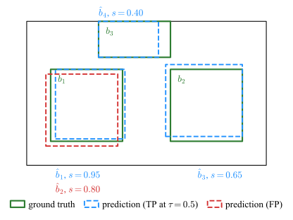
Example 25.1 (Box matching at IoU \(\tau =0.5\)): A small image (Fig. 25.3) contains three ground-truth boxes \(b_1,b_2,b_3\) and four predictions \(\hat b_1,\ldots ,\hat b_4\) sorted by descending confidence. The matrix of pairwise IoUs (zero entries omitted) is
\[ \begin {array}{c|c|ccc} & \text {score} & b_1 & b_2 & b_3 \\\hline \hat b_1 & 0.95 & 0.87 & \cdot & \cdot \\ \hat b_2 & 0.80 & 0.77 & \cdot & \cdot \\ \hat b_3 & 0.65 & \cdot & 0.82 & \cdot \\ \hat b_4 & 0.40 & \cdot & \cdot & 0.83 \end {array} \]
Apply the greedy descending-confidence rule at \(\tau =0.5\): classify each prediction as TP or FP and identify any FN.
-
-
1. Walk the score-sorted list and match
Dispatch each prediction in descending-confidence order, letting it claim its highest-IoU still-unclaimed ground truth:
rank prediction score best GT IoU decision 1 \(\hat b_1\) 0.95 \(b_1\) 0.87 TP – claims \(b_1\) 2 \(\hat b_2\) 0.80 \(b_1\) 0.77 FP – duplicate, \(b_1\) already claimed 3 \(\hat b_3\) 0.65 \(b_2\) 0.82 TP – claims \(b_2\) 4 \(\hat b_4\) 0.40 \(b_3\) 0.83 TP – claims \(b_3\) -
2. Final counts: TP\(=3\), FP\(=1\), FN\(=0\) (every ground truth was claimed). The per-rank labels TP, FP, TP, TP are exactly the input of Example 25.2 below, which integrates them into AP.
-
25.2.2 Non-Maximum Suppression (NMS)
Table 25.1 contrasts box matching and NMS.
|
NMS |
Box matching \(+\) labeling |
|
|
When |
inference time (every run) |
evaluation time (computing metrics) |
|
Needs ground truth? |
no |
yes |
|
IoU compares |
prediction vs. prediction (\(\hat b_i\) vs. \(\hat b^{*}\)) |
prediction vs. ground truth (\(\hat b_i\) vs. \(b_j\)) |
|
Threshold |
\(\tau _{\text {NMS}}\) |
\(\tau \) |
|
Produces |
the clean predicted-box list |
TP/FP/FN counts |
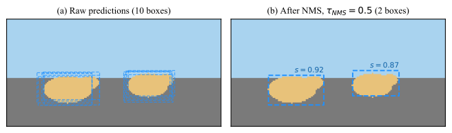
At inference time the detector must return a clean box list rather than a labeled one, so it deletes the duplicates outright. Non-maximum suppression (NMS, used by one-stage detectors such as YOLO, Sec. 25.3) does this with the same greedy descending-confidence sweep as the matching rule, except each prediction is compared against the boxes already kept rather than against the ground truth:
-
1. Sort the class-\(c\) predictions by descending confidence scores \(\{s_i\}\), as in Stage 1.
-
2. Pop the highest-scoring box \(\hat b^{*}\) and keep it; remove every remaining prediction \(\hat b_i\) with \(\text {IoU}(\hat b_i,\hat b^{*}) > \tau _{\text {NMS}}\). Predictions with \(\text {IoU}(\hat b_i,\hat b^{*}) \le \tau _{\text {NMS}}\) overlap \(\hat b^{*}\) too little to be duplicates and stay in the pool as candidates for separate objects.
-
3. Repeat on what is left.
The NMS threshold \(\tau _{\text {NMS}}\) (commonly \(0.5\)–\(0.7\)) trades the two failure modes: too low merges genuinely adjacent objects (two pedestrians become one box), too high leaves duplicates. Figure 25.4 illustrates the effect on a two-sheep scene.
25.2.3 Precision–recall curve
With every prediction labeled TP or FP and the FN count fixed (Stage 1), the only remaining freedom is how many predictions to admit. Each predicted box has a confidence \(s\). Sweeping a cut-off \(s_0\) from \(1\) down to \(0\) and admitting only predictions with \(s\ge s_0\) produces a sequence of (precision, recall) pairs:
\(\seteqnumber{0}{25.}{0}\)\begin{equation} \text {Pr}(s_0) = \frac {\text {TP}(s_0)}{\text {TP}(s_0)+\text {FP}(s_0)} , \qquad \text {Re}(s_0) = \frac {\text {TP}(s_0)}{\text {TP}(s_0)+\text {FN}} . \end{equation}
Plotting Pr vs. Re gives the precision–recall curve at IoU threshold \(\tau \).
25.2.4 Average precision
A whole curve is awkward to compare across models, so Stage 3 reduces it to a single scalar. Average Precision (AP) at IoU threshold \(\tau \) is the area under the (interpolated) precision–recall curve,
\(\seteqnumber{0}{25.}{1}\)\begin{equation} \text {AP}_\tau \;=\; \int _0^1 \text {Pr}_{\text {int}}(r)\,\mathrm {d}r , \qquad \text {Pr}_{\text {int}}(r) \;=\; \max _{r'\ge r}\text {Pr}(r') , \label {eq-dlarch-ap} \end{equation}
where the interpolation \(\text {Pr}_{\text {int}}\) replaces precision at recall \(r\) by the highest precision attained at any recall \(r'\ge r\), removing the zig-zag of the raw curve.
Two integration conventions coexist:
-
• 11-point interpolation (Pascal VOC, Sec. 24.3, pre-2010): average \(\text {Pr}_{\text {int}}\) over \(r\in \{0,0.1,\ldots ,1.0\}\).
-
• All-point interpolation (VOC post-2010, COCO, Sec. 24.3): integrate over all distinct recall values.
The two yield slightly different numbers and are not directly comparable.
-
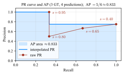
Example 25.2 (AP from a small detection table): Reusing the four predictions from Example 25.1 (three ground-truth boxes; TP, FP, TP, TP at descending scores \(0.95, 0.80, 0.65, 0.40\) at IoU threshold \(\tau =0.5\)):
\[ \begin {array}{c|c|c|c|c} \text {rank} & \text {score} & \text {TP/FP} & \text {cumulative TP} & \text {cumulative FP}\\\hline 1 & 0.95 & \text {TP} & 1 & 0\\ 2 & 0.80 & \text {FP} & 1 & 1\\ 3 & 0.65 & \text {TP} & 2 & 1\\ 4 & 0.40 & \text {TP} & 3 & 1 \end {array} \]
Compute AP using all-point interpolation.
-
-
1. Build the (recall, precision) points
With three ground-truth boxes (\(\text {TP}+\text {FN}=3\)) the recall axis advances by \(1/3\) per TP. For each rank \(k\), using the cumulative TP/FP counts from the table,
\[ r_k = \frac {\text {cum TP}_k}{\text {TP}+\text {FN}}, \qquad p_k = \frac {\text {cum TP}_k}{\text {cum TP}_k + \text {cum FP}_k} . \]
For instance at rank \(k=3\) (score \(s=0.65\)) the table gives \(\text {cum TP}_3=2\) and \(\text {cum FP}_3=1\), so
\[ r_3 = \tfrac {2}{3}, \qquad p_3 = \tfrac {2}{2+1} = \tfrac {2}{3} . \]
Applying the same formulas to all four ranks gives the (recall, precision) points
\[ (1/3,\,1.00),\;(1/3,\,1/2),\;(2/3,\,2/3),\;(1,\,3/4) , \]
shown as red dots in Fig. 25.5, each labelled by its admission score \(s\).
-
2. Interpolate
Interpolated precision is the running maximum of precision over recalls \(r'\ge r\): the largest precision attained is \(1\) at \(r=1/3\) and the maximum at recall \(\ge 2/3\) is \(3/4\) (at \(r=1\), since \(3/4>2/3\)), so
\[ \text {Pr}_{\text {int}}(r) = \begin {cases}1 & 0\le r\le 1/3 ,\\ 3/4 & 1/3 < r\le 1 ,\end {cases} \]
plotted as the blue step in Fig. 25.5.
-
3. Integrate
The integral, i.e. the shaded area in Fig. 25.5, evaluates to
\[ \text {AP} \;=\; \tfrac 13\cdot 1 + \tfrac 23\cdot \tfrac 34 \;=\; \tfrac 13 + \tfrac 12 \;=\; \tfrac {5}{6}\approx 0.83 . \]
-
25.2.5 mAP and COCO-style mAP
Stage 3 produces one AP per class at one IoU threshold; the final stage averages those into the single number reported on a benchmark. Mean Average Precision (mAP) at IoU threshold \(\tau \) is the arithmetic mean of per-class \(\text {AP}_{\tau ,c}\) over the \(C\) classes:
\(\seteqnumber{0}{25.}{2}\)\begin{equation} \text {mAP}_\tau \;=\; \frac {1}{C}\sum _{c=1}^C \text {AP}_{\tau ,c} , \label {eq-dlarch-map} \end{equation}
where \(\text {AP}_{\tau ,c}\) is computed exactly as in Eq. 25.2 but restricting predictions and ground-truth boxes to class \(c\). Averaging over classes treats every class as equally important regardless of its frequency in the dataset: a model that nails the dominant class but misses every rare class will still score poorly. (To compute one \(\text {AP}_{\tau ,c}\), sweep the per-class predictions sorted by score, accumulate per-class TP/FP/FN, and integrate the resulting per-class PR curve.) COCO introduced a stricter metric that averages over IoU thresholds as well,
\(\seteqnumber{0}{25.}{3}\)\begin{equation} \text {mAP}_{[.5:.95]} \;=\; \frac {1}{10}\sum _{\tau \in \{0.50,0.55,\ldots ,0.95\}}\text {mAP}_\tau , \label {eq-dlarch-map-coco} \end{equation}
which rewards tight localization: a model that overlaps ground-truth by \(0.5\) scores well at \(\tau =0.5\) but collapses at \(\tau =0.95\).
AP is per-class at one IoU threshold; mAP averages AP over classes; mAP@[.5:.95] also averages over \(10\) IoU thresholds and is the headline number on COCO.
25.3 Architecture
All detection networks share the same skeleton: a CNN backbone produces a dense feature map, i.e. a low-resolution \(H'\times W'\times C\) tensor whose \((h,w)\) cell carries a learned \(C\)-dimensional descriptor of the input-image patch that maps to that location; one or more prediction heads turn each feature-map cell into candidate boxes with an objectness (the class-agnostic probability that the box contains any object versus background) and a class distribution; NMS (Sec. 25.2) prunes duplicates. The per-(box, class) score \(s\) that the evaluator sees is built from these two: in one-stage detectors typically \(s = \text {objectness}\times \text {class probability}\), in two-stage detectors objectness is the score the first stage uses to keep proposals and \(s\) is the class probability output by the second-stage classifier. Families differ in how many passes it takes to get from the feature map to the final box list.
The two practically relevant families are then:
-
• Two-stage detectors (R-CNN family: Faster R-CNN, Mask R-CNN): stage 1 emits region proposals, stage 2 classifies and refines each.
-
• One-stage detectors (YOLO, SSD, RetinaNet): a single forward pass predicts boxes and classes densely over the feature grid.
A third family, transformer-based detectors (DETR and successors), predicts the whole set of boxes in one forward pass without anchors and without NMS, trading longer training for a simpler inference pipeline; it is increasingly competitive but not yet the practitioner default.
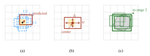
Three detection-specific terms used below (see Fig. 25.6):
-
• Anchor box: a fixed reference rectangle of preset size and aspect ratio, tiled at every feature-map location. The network predicts an offset and a score for each anchor instead of regressing a box from scratch.
-
• Anchor-free head: predicts box center and size \((w,h)\) directly per feature-map cell, with no reference rectangles.
-
• Region proposal: a candidate box with an objectness score but no class yet, emitted by a first stage and fed to a second stage that classifies and refines it.
R-CNN family The modern reference is Faster R-CNN: the backbone produces a feature map once per image; a small sub-network slides over that feature map and emits a fixed pool of anchor-based region proposals with objectness scores; the top-scoring proposals are passed to a second-stage head that outputs a class label and a refined box per proposal. Mask R-CNN adds a parallel head that produces a binary mask per proposal, making the same network usable for instance segmentation (Ch. 24). Practical profile: highest accuracy on COCO-style benchmarks, slowest per image, the default when latency is not the bottleneck or when masks or keypoints are also required.
YOLO YOLO (“You Only Look Once”) treats detection as a single dense regression problem. A CNN backbone reduces the input to a coarse feature grid (e.g. \(13\times 13\)); each grid cell predicts a small fixed number of candidate boxes together with an objectness score and a class distribution, all in one forward pass. Low-confidence boxes are discarded and overlapping survivors are pruned per class by NMS (Sec. 25.2). Modern variants predict at multiple feature-map resolutions so that small, medium and large objects share the same backbone, and recent open-source releases (Ultralytics YOLOv8/v11) ship anchor-free heads and one-line fine-tuning from COCO weights. Practical profile: real-time on commodity GPUs and edge devices, the practitioner default for deployment, accuracy now close to two-stage on modern variants.
Summary
Architecture choice in one line:
-
• Real-time or edge deployment \(\to \) one-stage (YOLO).
-
• Maximum accuracy, or masks/keypoints also needed \(\to \) two-stage (Mask R-CNN).
-
• Simpler pipeline, no NMS tuning, willing to train longer \(\to \) transformer (DETR).
25.4 Notes
Hyperparameters
Architecture-specific hyperparameters are to be tuned (out of scope in this chapter), e.g.: for anchor-based detectors, the number, scales and aspect ratios of the anchor presets; for two-stage detectors, the number of proposals kept after stage 1; for one-stage detectors, the input resolution and the number of feature-map scales.
Reporting performance
-
• Reporting a single IoU threshold (mAP@.5) when comparing to COCO-era methods. Always include mAP@[.5:.95] alongside mAP@.5.
-
• Mixing 11-point and all-point AP across papers and quoting the numbers as comparable. They are not.
Object size influence
Small objects are punished by IoU: a \(5\times 5\) ground-truth box with a one-pixel boundary error already loses \(\sim 36\%\) of IoU. Reporting \(\text {AP}_{\text {small}}\), \(\text {AP}_{\text {medium}}\), \(\text {AP}_{\text {large}}\) separately (COCO convention) is informative whenever object size varies across the dataset.
Further Reading
Convolutional Neural Networks (Course 4 of the Deep Learning Specialization), especially C4W3 (object detection)
-
• WPI Demo
-
• Web AI Demo of the library that allows you to run modern deep learning models directly in your web browser (accessed 25-May-2026)