The axis is where a plot is most often quietly wrong, because the same choice is legitimate for one encoding and misleading for another.
7.1 The zero baseline
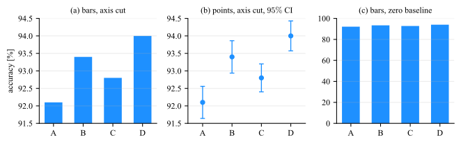
Whether an axis must include zero is decided by the encoding, not by convention. A bar encodes its value as a length measured from the baseline. A line encodes position, so cutting the axis rescales the whole
picture uniformly and the reader can see the axis labels. Fig. 7.1 is the bar case and Fig. 7.2 the position case.
Figure 7.1: Four test accuracies, \(92.1\), \(93.4\), \(92.8\) and \(94.0\) percent. (a) With the axis cut at \(91.5\), the bar for \(D\) is \(4.2\) times the length of the bar for \(A\), though the values differ by \(2\%\):
an exaggeration of a factor of \(4.1\). (b) The same numbers as points, on the same cut axis as (a), with the \(95\%\) confidence interval of each over its \(5\) folds. The cut is legitimate here and not in (a), because a point is at a
position while a bar is a length measured from the baseline. The panel also reports what neither bar panel can: \(B\) at \(93.40 \pm 0.46\) and \(D\) at \(94.00 \pm 0.43\) are separated from \(A\) at \(92.10 \pm 0.46\), and
\(C\) at \(92.80 \pm 0.40\) is not. (c) The same numbers as bars on a zero baseline, where the four models are correctly seen to be nearly tied.
A cut bar chart is not a style choice
Panel (a) of Fig. 7.1 is the most common misleading chart in circulation, and it is usually produced by accident: many libraries auto-scale the axis to the data range,
so cutting the baseline is what happens when nothing is specified. Any bar chart whose baseline is not zero should be treated as an error to be fixed, not a decision to be defended.
If the differences are too small to see on a zero baseline and they matter, plot the differences themselves, with their confidence intervals, on a zero that means no difference.
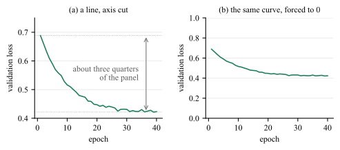
The rule is about bars, and it does not run backwards: an axis that includes zero is not automatically the safer one. Fig. 7.2 is the same argument from the other side, on a
quantity whose marks encode position.
Figure 7.2: A \(40\)-epoch validation loss, drawn twice. (a) The marks encode position, the axis is labeled, the decay and the plateau are both readable, and the limits are chosen so that the curve fills the marked \(76\%\) of
the panel. (b) The identical curve forced onto \(0\) to \(1\).
Forcing zero onto panel (b) does not make it honest, it deletes the finding: the plateau is left with is less than the separation at which a reader resolves anything at all. Nothing is gained in exchange, because no mark in the
panel is a length measured from the baseline, so there is no length for the cut to distort.
How far to cut
A cut is a choice of limits, not just a decision to leave zero out. Choose them so that the data fill about two thirds to three quarters of the panel.
7.2 Cumulative totals
The baseline is not the only way a chart can be exactly right about its numbers and wrong about the question. A running total is monotone by construction: it cannot fall, whatever the process underneath it does, so it always
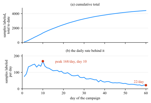
draws a rising curve. Presented as evidence that an effort is working, it is evidence of nothing. Fig. 7.3 plots one record both ways.
Figure 7.3: A \(60\)-day labeling campaign, plotted as a total and as a rate. (a) The running total climbs to \(4429\) samples and rises on every one of its \(59\) steps, since a cumulative curve cannot do anything else. (b)
The daily rate that produced it: a peak of \(168\) per day on day \(10\), falling to \(22\) per day by day \(60\), which is \(13\%\) of the peak. The first week contributed \(20\%\) of the total and the last week \(4\%\). Both
panels are exact, and only (b) answers whether the campaign is still working.
Plot the quantity the question is about!
7.3 Aspect ratio
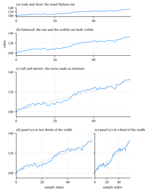
The physical shape of the axes changes the slope a reader perceives, and slope is how a line chart is read. Fig. 7.4 draws one series five times with identical axis limits: the
first three change the height of the axes, and the last two repeat the third of them at two thirds and at a third of its width.
Figure 7.4: One series, one pair of axis limits, five axes shapes. The median segment of the line meets the horizontal at \(7.0^{\circ }\) in (a), \(17.5^{\circ }\) in (b) and \(32.2^{\circ }\) in (c), so the slope the reader
perceives grows with the height of the axes. Panels (d) and (e) are (c) narrowed to two thirds and to a third of its width, which delivers \(43.4^{\circ }\) and \(63.7^{\circ }\).
Ad hoc Cleveland’s rule of thumb is to bank to \(45^{\circ }\): choose the aspect ratio so that the typical line segment meets the horizontal near \(45^{\circ }\), since that is where a change in slope is easiest
to detect.
7.4 Ticks and labels
Easy numbers
Ticks at \(1\), \(2\), \(5\), \(10\) and their mulitplications/powers, never at the \(7\) or \(13\) an algorithm sometimes lands on.
Labeled axes
Every axis names a quantity and a unit. A number without a unit is not a measurement.
Compress offset
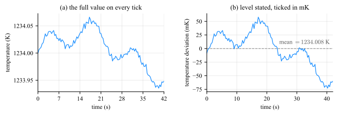
A quantity far from zero has its level stated on the panel and its deviation ticked in a unit sized to the drift. An offset parked in a corner box, or spelled out on every tick, both leave the reader doing arithmetic.
Fig. 7.5(a) does what a reader normally asks for and puts the full value on every tick, and this record will not support it: six digits a label to report a drift of
\(131\) mK, so the level is printed five times over, the quantity the figure is about is carried by the last two digits, and the ticks fall at \(7\) s. State the level on the panel, and tick the deviation from it in a unit sized
to the drift, which is panel (b).
Figure 7.5: (a) The full value on every tick: the axis runs \(1233.90\) to \(1234.10\) K in steps of \(0.05\) K, which is six digits a label of which only the last two carry the drift, and the ticks fall at \(7\) s.
(b) The same record with the level subtracted and the deviation from it ticked in millikelvin: ticks at \(10\) s and \(25\) mK, every one of them a small round number. Zero on this axis is the mean and nothing else,
the dashed line marks it and names it in full, \(1234.008\) K, so any mark on the panel converts back to an absolute temperature, and the record is seen to run \(-73\) to \(+58\) mK about it.
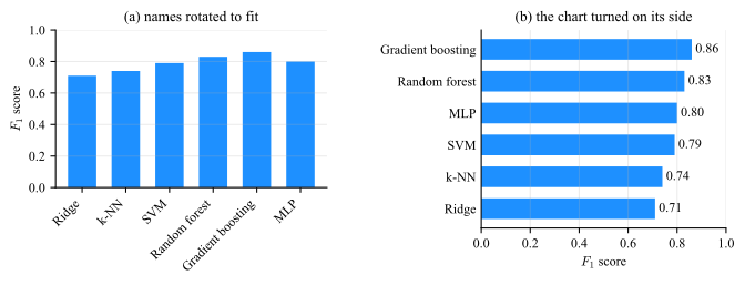
And treat rotated tick labels as a diagnostic rather than a solution: if the label names do not fit horizontally, the chart wants to be horizontal.
Rotating a label is not a style preference (Fig. 7.6). The six names are the same in both panels and so are the six numbers; what changes is where the names are kept. Tilted
under the axis they claim \(18.3\) mm of a \(66\) mm figure, which is \(28\%\) of its height taken out of the bars, and the reader still has to read them at an angle. Turned on their side they claim
\(22.8\) mm of width, which comes out of the margin rather than the panel, and the same figure gives the bars \(47.2\) mm of height instead of \(37.6\).
Figure 7.6: Six \(F_1\) scores drawn twice in one figure box with nothing changed but where the category names are kept. (a) Names tilted at \(45^{\circ }\) to fit under a vertical axis. (b) The chart turned on its side.
7.5 Legends
A series has to be named somewhere, and there are only two approaches to put the name; the two differ in which of the two reading operations of Sec. 4.1 the reader is
made to perform.
• A boxed legend is a key set apart from the data, mapping a color or a line style to a name. Reading it is a table look-up, and it is a look-up per mark: the reader carries a
color/style to the box, finds the matching key, carries the name back, and repeats it for the next series.
• An end-of-line label is the name set at the end of the series it belongs to, in that series’ color. There is nothing to carry anywhere, because the name is already where the reader is
looking.
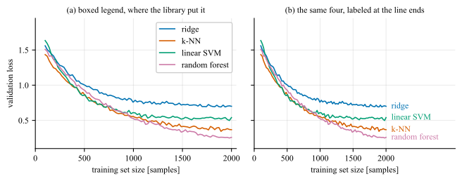
Figure 7.7: Learning curves for four models on identical axes, named two ways. (a) A boxed legend at the position the library chose: it spends \(15\%\) of the panel on the key, and its entries are in the order the series were
plotted, which is not the order they arrive in at the right edge, so \(2\) of the \(4\) are out of place and the reader re-sorts on every look-up. (b) The same four named where they end. No panel area is spent, no color has to be
carried anywhere, and the names survive a gray print and a color vision deficiency simulation because there the name identifies the curve and the color only decorates it.
Three consequences, in the order they usually matter.
Label directly whenever there is room. It removes the look-up entirely.
Where a box is unavoidable, order it to match the page. Sort its entries to match the vertical order of the series at the edge where the reader meets them, and place it over a region carrying no data.
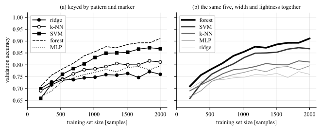
What the key is made of decides what the look-up costs. A key is read no faster than the channel it maps. Dash patterns and marker shapes are nominal: the entries have no order among them, so each is matched
glyph by glyph, and the match is made again wherever the curves cross, which is exactly where the glyphs are hardest to tell apart. Line width and lightness are ordered: moved together they turn the key into a sequence,
read once and then predicted, and its entries come out in the order the curves appear on the page, which is the previous rule obtained for nothing. Fig. 7.8 is one record
under both.
Figure 7.8: Five plot with a boxed legend in both panels. (a) Keyed by dash pattern and marker shape. The five entries have no order among them. (b) The same five keyed by one ladder, line width from \(2.6\) to
\(0.7\) pt and gray from \(0.00\) to \(0.72\).
The one place redundancy is worth its ink
Encoding a quantity twice is normally waste (Sec. 11), and panel (b) does it on purpose: the rank of a series is in its width and in its lightness at once.
With \(6+\) series, neither form works. End labels start to collide wherever the series converge, a box with a dozen keys is a second figure to read before the first one can be, and no ladder has a dozen separable steps
either. That is the point at which the answer is small multiples (Sec. 7.6) or highlighting one series against gray (Fig. 5.12), not a smaller font.
7.6 Many plots at once
Goal: What does a reader do with ten series that will not fit on one axis?
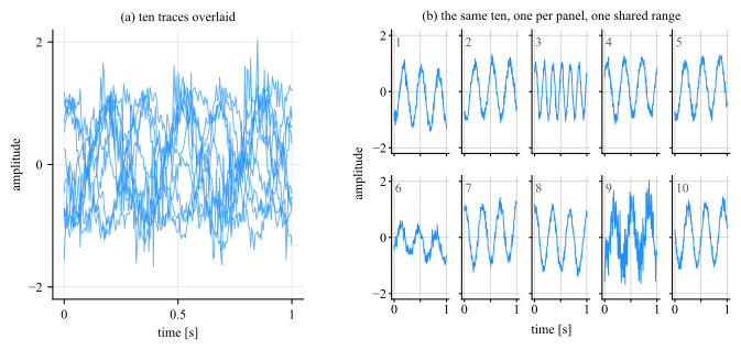
Legend won’t help. Stop drawing one plot and draw many: one panel per series, laid out as a grid, every panel on the same range. The grid is called small multiples. Fig. 7.9 is the overlay beside its replacement.
Figure 7.9: Ten recordings from one process. (a) Overlaid: the envelope is readable and nothing else is. (b) The same ten as small multiples, one panel each, on one linked range. Three of the ten are not like the
rest, in three different ways: trace \(3\) runs at \(6\) Hz against the \(3\) Hz of the others, trace \(6\) has \(0.55\) of their amplitude, and trace \(9\) carries \(4.1\) times their noise. Not one of the three can be
found in (a).
•One range, set once. Give the panels a single range on both axes and link them, so that the range is a property of the block rather than ten separate decisions. Per-panel
autoscaling is the default in most libraries, and it produces ten plots that look like a comparison and are not one.
•Values on the outer edge only. The left column carries the \(y\) values and the bottom row the \(x\) values, and one label of each names the block. Ten copies of one axis is nine
copies of ink, which is Sec. 11 applied to a layout.
•Rule every panel, at the ticks it keeps. A panel stripped of its scale reports a shape and no quantity, exactly as a close-up does (Sec. 7.7), and the separation still has to clear the limit of Sec. 7.8 at the panel’s reduced size.
Sec. 4 to answer “where is this one among the rest” at a glance, and can be repeated across a row of panels to walk through several. Fig. 5.12 is the comparison, on twelve series that an overlay cannot separate.
7.7 Close-ups
One axis range cannot always serve both the extent of a record and a feature inside it. A transient a few milliseconds wide, drawn across a panel that covers seconds, gets a fraction of a millimeter of the page whatever the aspect
ratio, and no amount of care with the ticks recovers it. The answer is a second view at a second scale, and it comes in two forms.
• An inset: a small second axes drawn inside the panel, in a region that carries no data. It keeps the overview and the detail in one frame, and it costs nothing but the space it
occupies.
• A broken-out panel: the same window as a full panel beside the overview. It is the answer when the parent has no free corner, when the zoom needs its own axis labels, or when the
required magnification is large enough that a small inset would not resolve the feature anyway.
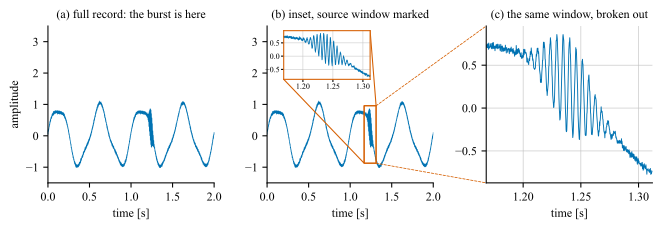
Figure 7.10: A \(2\) s record sampled at \(5\) kHz, carrying a \(180\) Hz burst on a \(2\) Hz carrier, a frequency ratio of \(90\). (a) The full record: the burst is at \(1.24\) s, it is the only
thing the record is about. (b) An inset over the \(144\) ms window that contains it, a magnification of \(14\), with the source window boxed on the parent and connected to the inset so the reader can locate what was
magnified. (c) The same samples as a panel of their own, which is what the window needs when the parent has no room.
•Mark the source window with a rectangle on the parent panel, and connect the rectangle to the view it produced.
•Keep the ticks on the close-up, and rule it at them. A zoom without a scale shows a shape and reports no quantity, and the reader has no way to tell a \(10\)-fold magnification
from a \(100\)-fold one. Ticks are the minimum; the grid at those ticks is what turns the magnified shape into values the reader can take off the page (Sec. 7.8), and
a close-up is read for values rather than for where the feature sits.
•Put the inset where there is no data. If the panel has no empty region, that is the signal to break the view out into its own panel rather than to cover the trace with it.
7.8 Size and gridlines
Goal: How tall must a panel be, and how finely may it be ruled?
Two rules for the grid
• Rule the panel. The grid is the route from a mark to a number, and adding one improved accuracy at every size measured.
• Do not shrink a panel below the height at which its scale can be read.
• Do not rule it more finely than the reader can resolve.
• At a typical rendering of \(96\) pixels per inch that is a height of about \(2\) cm and a gridline separation of at least \(2\) mm, both measured on the printed page rather than
on the screen the figure was authored on.
Both numbers are measured rather than chosen, and two results are what the measurement leaves for use.4
• On a \(0\) to \(100\) scale, gridlines every \(10\) or \(20\) units beat gridlines every \(50\) or \(100\).
• Not usefull once the lines fall closer together than the reader can separate them, which is about \(8\) pixels, or \(2\) mm at final size.
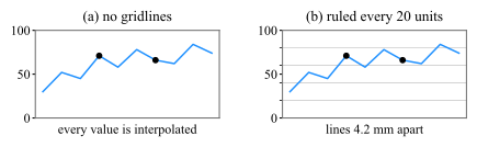
The default is often no grid at all, or a line every \(50\) units, and both leave the reader interpolating a value across half the panel. Fig. 7.11 is that case beside its fix, at
one panel size, so the ruling is the only thing that changes between the two.
Figure 7.11: One series on a \(0\) to \(100\) scale, with the two values a reader is asked to compare, \(71\) and \(66\), marked. Both panels are \(80\) pixels tall, that is \(21.2\) mm at \(96\) pixels per inch, and
they differ in nothing but the ruling. (a) No gridlines by default. (b) The same panel ruled every \(20\) units, which is \(4.2\) mm at this height and twice the \(2.1\) mm the eye needs to keep two lines apart: each
marked value now sits against a line instead of being estimated.
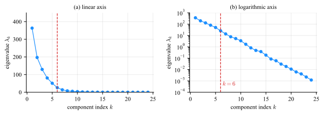
When a quantity spans several orders of magnitude, a linear axis shows the largest decade and compresses everything else onto the baseline (Fig. 7.12).
Figure 7.12: An eigenvalue spectrum spanning five and a half decades, from \(363\) to \(0.0012\). (a) On a linear axis, \(15\) of the \(24\) eigenvalues fall below \(1\%\) of the largest and are pinned to the baseline,
indistinguishable from one another and from zero. (b) On a logarithmic axis, the same spectrum is a straight line, which identifies the decay as exponential, and the change of regime at the dashed line becomes something the reader
can locate rather than guess.
No zero or negative values
A log axis cannot show zero or negative values, so a curve that reaches zero needs a different treatment