Plotting

\(\newcommand{\footnotename}{footnote}\) \(\def \LWRfootnote {1}\) \(\newcommand {\footnote }[2][\LWRfootnote ]{{}^{\mathrm {#1}}}\) \(\newcommand {\footnotemark }[1][\LWRfootnote ]{{}^{\mathrm {#1}}}\) \(\let \LWRorighspace \hspace \) \(\renewcommand {\hspace }{\ifstar \LWRorighspace \LWRorighspace }\) \(\newcommand {\TextOrMath }[2]{#2}\) \(\newcommand {\mathnormal }[1]{{#1}}\) \(\newcommand \ensuremath [1]{#1}\) \(\newcommand {\LWRframebox }[2][]{\fbox {#2}} \newcommand {\framebox }[1][]{\LWRframebox } \) \(\newcommand {\setlength }[2]{}\) \(\newcommand {\addtolength }[2]{}\) \(\newcommand {\setcounter }[2]{}\) \(\newcommand {\addtocounter }[2]{}\) \(\newcommand {\arabic }[1]{}\) \(\newcommand {\number }[1]{}\) \(\newcommand {\noalign }[1]{\text {#1}\notag \\}\) \(\newcommand {\cline }[1]{}\) \(\newcommand {\directlua }[1]{\text {(directlua)}}\) \(\newcommand {\luatexdirectlua }[1]{\text {(directlua)}}\) \(\newcommand {\protect }{}\) \(\def \LWRabsorbnumber #1 {}\) \(\def \LWRabsorbquotenumber "#1 {}\) \(\newcommand {\LWRabsorboption }[1][]{}\) \(\newcommand {\LWRabsorbtwooptions }[1][]{\LWRabsorboption }\) \(\def \mathchar {\ifnextchar "\LWRabsorbquotenumber \LWRabsorbnumber }\) \(\def \mathcode #1={\mathchar }\) \(\let \delcode \mathcode \) \(\let \delimiter \mathchar \) \(\def \oe {\unicode {x0153}}\) \(\def \OE {\unicode {x0152}}\) \(\def \ae {\unicode {x00E6}}\) \(\def \AE {\unicode {x00C6}}\) \(\def \aa {\unicode {x00E5}}\) \(\def \AA {\unicode {x00C5}}\) \(\def \o {\unicode {x00F8}}\) \(\def \O {\unicode {x00D8}}\) \(\def \l {\unicode {x0142}}\) \(\def \L {\unicode {x0141}}\) \(\def \ss {\unicode {x00DF}}\) \(\def \SS {\unicode {x1E9E}}\) \(\def \dag {\unicode {x2020}}\) \(\def \ddag {\unicode {x2021}}\) \(\def \P {\unicode {x00B6}}\) \(\def \copyright {\unicode {x00A9}}\) \(\def \pounds {\unicode {x00A3}}\) \(\let \LWRref \ref \) \(\renewcommand {\ref }{\ifstar \LWRref \LWRref }\) \( \newcommand {\multicolumn }[3]{#3}\) \(\require {textcomp}\) \( \newcommand {\abs }[1]{\lvert #1\rvert } \) \( \DeclareMathOperator {\sign }{sign} \) \(\newcommand {\intertext }[1]{\text {#1}\notag \\}\) \(\let \Hat \hat \) \(\let \Check \check \) \(\let \Tilde \tilde \) \(\let \Acute \acute \) \(\let \Grave \grave \) \(\let \Dot \dot \) \(\let \Ddot \ddot \) \(\let \Breve \breve \) \(\let \Bar \bar \) \(\let \Vec \vec \) \(\newcommand {\bm }[1]{\boldsymbol {#1}}\) \(\require {physics}\) \(\newcommand {\LWRphystrig }[2]{\ifblank {#1}{\textrm {#2}}{\textrm {#2}^{#1}}}\) \(\renewcommand {\sin }[1][]{\LWRphystrig {#1}{sin}}\) \(\renewcommand {\sinh }[1][]{\LWRphystrig {#1}{sinh}}\) \(\renewcommand {\arcsin }[1][]{\LWRphystrig {#1}{arcsin}}\) \(\renewcommand {\asin }[1][]{\LWRphystrig {#1}{asin}}\) \(\renewcommand {\cos }[1][]{\LWRphystrig {#1}{cos}}\) \(\renewcommand {\cosh }[1][]{\LWRphystrig {#1}{cosh}}\) \(\renewcommand {\arccos }[1][]{\LWRphystrig {#1}{arcos}}\) \(\renewcommand {\acos }[1][]{\LWRphystrig {#1}{acos}}\) \(\renewcommand {\tan }[1][]{\LWRphystrig {#1}{tan}}\) \(\renewcommand {\tanh }[1][]{\LWRphystrig {#1}{tanh}}\) \(\renewcommand {\arctan }[1][]{\LWRphystrig {#1}{arctan}}\) \(\renewcommand {\atan }[1][]{\LWRphystrig {#1}{atan}}\) \(\renewcommand {\csc }[1][]{\LWRphystrig {#1}{csc}}\) \(\renewcommand {\csch }[1][]{\LWRphystrig {#1}{csch}}\) \(\renewcommand {\arccsc }[1][]{\LWRphystrig {#1}{arccsc}}\) \(\renewcommand {\acsc }[1][]{\LWRphystrig {#1}{acsc}}\) \(\renewcommand {\sec }[1][]{\LWRphystrig {#1}{sec}}\) \(\renewcommand {\sech }[1][]{\LWRphystrig {#1}{sech}}\) \(\renewcommand {\arcsec }[1][]{\LWRphystrig {#1}{arcsec}}\) \(\renewcommand {\asec }[1][]{\LWRphystrig {#1}{asec}}\) \(\renewcommand {\cot }[1][]{\LWRphystrig {#1}{cot}}\) \(\renewcommand {\coth }[1][]{\LWRphystrig {#1}{coth}}\) \(\renewcommand {\arccot }[1][]{\LWRphystrig {#1}{arccot}}\) \(\renewcommand {\acot }[1][]{\LWRphystrig {#1}{acot}}\) \(\require {cancel}\) \(\newcommand {\underuparrow }[1]{{\underset {\uparrow }{#1}}}\) \(\DeclareMathOperator *{\argmax }{argmax}\) \(\DeclareMathOperator *{\argmin }{arg\,min}\) \(\def \E [#1]{\mathbb {E}\!\left [ #1 \right ]}\) \(\def \Var [#1]{\operatorname {Var}\!\left [ #1 \right ]}\) \(\def \Cov [#1]{\operatorname {Cov}\!\left [ #1 \right ]}\) \(\newcommand {\floor }[1]{\lfloor #1 \rfloor }\) \(\newcommand {\DTFTH }{ H \brk 1{e^{j\omega }}}\) \(\newcommand {\DTFTX }{ X\brk 1{e^{j\omega }}}\) \(\newcommand {\DFTtr }[1]{\mathrm {DFT}\left \{#1\right \}}\) \(\newcommand {\DTFTtr }[1]{\mathrm {DTFT}\left \{#1\right \}}\) \(\newcommand {\DTFTtrI }[1]{\mathrm {DTFT^{-1}}\left \{#1\right \}}\) \(\newcommand {\Ftr }[1]{ \mathcal {F}\left \{#1\right \}}\) \(\newcommand {\FtrI }[1]{ \mathcal {F}^{-1}\left \{#1\right \}}\) \(\newcommand {\Zover }{\overset {\mathscr Z}{\Longleftrightarrow }}\) \(\renewcommand {\real }{\mathbb {R}}\) \(\newcommand {\ba }{\mathbf {a}}\) \(\newcommand {\bb }{\mathbf {b}}\) \(\newcommand {\bc }{\mathbf {c}}\) \(\newcommand {\bd }{\mathbf {d}}\) \(\newcommand {\be }{\mathbf {e}}\) \(\newcommand {\bf }{\mathbf {f}}\) \(\newcommand {\bg }{\mathbf {g}}\) \(\newcommand {\bh }{\mathbf {h}}\) \(\newcommand {\bi }{\mathbf {i}}\) \(\newcommand {\bn }{\mathbf {n}}\) \(\newcommand {\bo }{\mathbf {o}}\) \(\newcommand {\bp }{\mathbf {p}}\) \(\newcommand {\bq }{\mathbf {q}}\) \(\newcommand {\br }{\mathbf {r}}\) \(\newcommand {\bs }{\mathbf {s}}\) \(\newcommand {\bt }{\mathbf {t}}\) \(\newcommand {\bu }{\mathbf {u}}\) \(\newcommand {\bv }{\mathbf {v}}\) \(\newcommand {\bw }{\mathbf {w}}\) \(\newcommand {\bx }{\mathbf {x}}\) \(\newcommand {\bxx }{\mathbf {xx}}\) \(\newcommand {\bxy }{\mathbf {xy}}\) \(\newcommand {\by }{\mathbf {y}}\) \(\newcommand {\byx }{\mathbf {yx}}\) \(\newcommand {\byy }{\mathbf {yy}}\) \(\newcommand {\bz }{\mathbf {z}}\) \(\newcommand {\bA }{\mathbf {A}}\) \(\newcommand {\bB }{\mathbf {B}}\) \(\newcommand {\bC }{\mathbf {C}}\) \(\newcommand {\bD }{\mathbf {D}}\) \(\newcommand {\bH }{\mathbf {H}}\) \(\newcommand {\bI }{\mathbf {I}}\) \(\newcommand {\bK }{\mathbf {K}}\) \(\newcommand {\bM }{\mathbf {M}}\) \(\newcommand {\bP }{\mathbf {P}}\) \(\newcommand {\bQ }{\mathbf {Q}}\) \(\newcommand {\bR }{\mathbf {R}}\) \(\newcommand {\bS }{\mathbf {S}}\) \(\newcommand {\bU }{\mathbf {U}}\) \(\newcommand {\bW }{\mathbf {W}}\) \(\newcommand {\bX }{\mathbf {X}}\) \(\newcommand {\bY }{\mathbf {Y}}\) \(\newcommand {\bZ }{\mathbf {Z}}\) \(\newcommand {\balpha }{\bm {\alpha }}\) \(\newcommand {\bth }{{\bm {\theta }}}\) \(\newcommand {\bepsilon }{{\bm {\epsilon }}}\) \(\newcommand {\bmu }{{\bm {\mu }}}\) \(\newcommand {\bgamma }{{\bm {\gamma }}}\) \(\newcommand {\bphi }{\bm {\phi }}\) \(\newcommand {\bOne }{\mathbf {1}}\) \(\newcommand {\bZero }{\mathbf {0}}\) \(\newcommand {\indFunc }{\mathbb {1}}\) \(\newcommand {\btx }{\tilde {\bx }}\) \(\newcommand {\loss }{\mathcal {L}}\) \(\newcommand {\score }{\mathcal {S}}\) \(\newcommand {\SSE }{\mathrm {SSE}}\) \(\newcommand {\SST }{\mathrm {SST}}\) \(\newcommand {\SSR }{\mathrm {SSR}}\) \(\newcommand {\MSE }{\mathrm {MSE}}\) \(\newcommand {\RMSE }{\mathrm {RMSE}}\) \(\newcommand {\toprule }[1][]{\hline }\) \(\let \midrule \toprule \) \(\let \bottomrule \toprule \) \(\def \LWRbooktabscmidruleparen (#1)#2{}\) \(\newcommand {\LWRbooktabscmidrulenoparen }[1]{}\) \(\newcommand {\cmidrule }[1][]{\ifnextchar (\LWRbooktabscmidruleparen \LWRbooktabscmidrulenoparen }\) \(\newcommand {\morecmidrules }{}\) \(\newcommand {\specialrule }[3]{\hline }\) \(\newcommand {\addlinespace }[1][]{}\) \(\newcommand {\LWRsubmultirow }[2][]{#2}\) \(\newcommand {\LWRmultirow }[2][]{\LWRsubmultirow }\) \(\newcommand {\multirow }[2][]{\LWRmultirow }\) \(\newcommand {\mrowcell }{}\) \(\newcommand {\mcolrowcell }{}\) \(\newcommand {\STneed }[1]{}\) \(\newcommand {\tcbset }[1]{}\) \(\newcommand {\tcbsetforeverylayer }[1]{}\) \(\newcommand {\tcbox }[2][]{\boxed {\text {#2}}}\) \(\newcommand {\tcboxfit }[2][]{\boxed {#2}}\) \(\newcommand {\tcblower }{}\) \(\newcommand {\tcbline }{}\) \(\newcommand {\tcbtitle }{}\) \(\newcommand {\tcbsubtitle [2][]{\mathrm {#2}}}\) \(\newcommand {\tcboxmath }[2][]{\boxed {#2}}\) \(\newcommand {\tcbhighmath }[2][]{\boxed {#2}}\) \(\require {colortbl}\) \(\let \LWRorigcolumncolor \columncolor \) \(\renewcommand {\columncolor }[2][named]{\LWRorigcolumncolor [#1]{#2}\LWRabsorbtwooptions }\) \(\let \LWRorigrowcolor \rowcolor \) \(\renewcommand {\rowcolor }[2][named]{\LWRorigrowcolor [#1]{#2}\LWRabsorbtwooptions }\) \(\let \LWRorigcellcolor \cellcolor \) \(\renewcommand {\cellcolor }[2][named]{\LWRorigcellcolor [#1]{#2}\LWRabsorbtwooptions }\) \(\newcommand {\tothe }[1]{^{#1}}\) \(\newcommand {\raiseto }[2]{{#2}^{#1}}\) \(\newcommand {\LWRsiunitxEND }{}\) \(\def \LWRsiunitxang #1;#2;#3;#4\LWRsiunitxEND {\ifblank {#1}{}{\num {#1}\degree }\ifblank {#2}{}{\num {#2}^{\unicode {x2032}}}\ifblank {#3}{}{\num {#3}^{\unicode {x2033}}}}\) \(\newcommand {\ang }[2][]{\LWRsiunitxang #2;;;\LWRsiunitxEND }\) \(\def \LWRsiunitxdistribunit {}\) \(\newcommand {\LWRsiunitxENDTWO }{}\) \(\def \LWRsiunitxprintdecimalsubtwo #1,#2,#3\LWRsiunitxENDTWO {\ifblank {#1}{0}{\mathrm {#1}}\ifblank {#2}{}{{\LWRsiunitxdecimal }\mathrm {#2}}}\) \(\def \LWRsiunitxprintdecimalsub #1.#2.#3\LWRsiunitxEND {\LWRsiunitxprintdecimalsubtwo #1,,\LWRsiunitxENDTWO \ifblank {#2}{}{{\LWRsiunitxdecimal }\LWRsiunitxprintdecimalsubtwo #2,,\LWRsiunitxENDTWO }}\) \(\newcommand {\LWRsiunitxprintdecimal }[1]{\LWRsiunitxprintdecimalsub #1...\LWRsiunitxEND }\) \(\def \LWRsiunitxnumplus #1+#2+#3\LWRsiunitxEND {\ifblank {#2}{\LWRsiunitxprintdecimal {#1}}{\ifblank {#1}{\LWRsiunitxprintdecimal {#2}}{\LWRsiunitxprintdecimal {#1}\unicode {x02B}\LWRsiunitxprintdecimal {#2}}}\LWRsiunitxdistribunit }\) \(\def \LWRsiunitxnumminus #1-#2-#3\LWRsiunitxEND {\ifblank {#2}{\LWRsiunitxnumplus #1+++\LWRsiunitxEND }{\ifblank {#1}{}{\LWRsiunitxprintdecimal {#1}}\unicode {x02212}\LWRsiunitxprintdecimal {#2}\LWRsiunitxdistribunit }}\) \(\def \LWRsiunitxnumpmmacro #1\pm #2\pm #3\LWRsiunitxEND {\ifblank {#2}{\LWRsiunitxnumminus #1---\LWRsiunitxEND }{\LWRsiunitxprintdecimal {#1}\unicode {x0B1}\LWRsiunitxprintdecimal {#2}\LWRsiunitxdistribunit }}\) \(\def \LWRsiunitxnumpm #1+-#2+-#3\LWRsiunitxEND {\ifblank {#2}{\LWRsiunitxnumpmmacro #1\pm \pm \pm \LWRsiunitxEND }{\LWRsiunitxprintdecimal {#1}\unicode {x0B1}\LWRsiunitxprintdecimal {#2}\LWRsiunitxdistribunit }}\) \(\newcommand {\LWRsiunitxnumscientific }[2]{\ifblank {#1}{}{\ifstrequal {#1}{-}{-}{\LWRsiunitxprintdecimal {#1}\times }}10^{\LWRsiunitxprintdecimal {#2}}\LWRsiunitxdistribunit }\) \(\def \LWRsiunitxnumD #1D#2D#3\LWRsiunitxEND {\ifblank {#2}{\LWRsiunitxnumpm #1+-+-\LWRsiunitxEND }{\mathrm {\LWRsiunitxnumscientific {#1}{#2}}}}\) \(\def \LWRsiunitxnumd #1d#2d#3\LWRsiunitxEND {\ifblank {#2}{\LWRsiunitxnumD #1DDD\LWRsiunitxEND }{\mathrm {\LWRsiunitxnumscientific {#1}{#2}}}}\) \(\def \LWRsiunitxnumE #1E#2E#3\LWRsiunitxEND {\ifblank {#2}{\LWRsiunitxnumd #1ddd\LWRsiunitxEND }{\mathrm {\LWRsiunitxnumscientific {#1}{#2}}}}\) \(\def \LWRsiunitxnume #1e#2e#3\LWRsiunitxEND {\ifblank {#2}{\LWRsiunitxnumE #1EEE\LWRsiunitxEND }{\mathrm {\LWRsiunitxnumscientific {#1}{#2}}}}\) \(\def \LWRsiunitxnumx #1x#2x#3x#4\LWRsiunitxEND {\ifblank {#2}{\LWRsiunitxnume #1eee\LWRsiunitxEND }{\ifblank {#3}{\LWRsiunitxnume #1eee\LWRsiunitxEND \times \LWRsiunitxnume #2eee\LWRsiunitxEND }{\LWRsiunitxnume #1eee\LWRsiunitxEND \times \LWRsiunitxnume #2eee\LWRsiunitxEND \times \LWRsiunitxnume #3eee\LWRsiunitxEND }}}\) \(\newcommand {\num }[2][]{\LWRsiunitxnumx #2xxxxx\LWRsiunitxEND }\) \(\newcommand {\si }[2][]{\mathrm {\gsubstitute {#2}{~}{\,}}}\) \(\def \LWRsiunitxSIopt #1[#2]#3{\def \LWRsiunitxdistribunit {\,\si {#3}}{#2}\num {#1}\def \LWRsiunitxdistribunit {}}\) \(\newcommand {\LWRsiunitxSI }[2]{\def \LWRsiunitxdistribunit {\,\si {#2}}\num {#1}\def \LWRsiunitxdistribunit {}}\) \(\newcommand {\SI }[2][]{\ifnextchar [{\LWRsiunitxSIopt {#2}}{\LWRsiunitxSI {#2}}}\) \(\newcommand {\numlist }[2][]{\text {#2}}\) \(\newcommand {\numrange }[3][]{\num {#2}\ \LWRsiunitxrangephrase \ \num {#3}}\) \(\newcommand {\SIlist }[3][]{\text {#2}\,\si {#3}}\) \(\newcommand {\SIrange }[4][]{\num {#2}\,#4\ \LWRsiunitxrangephrase \ \num {#3}\,#4}\) \(\newcommand {\tablenum }[2][]{\mathrm {#2}}\) \(\newcommand {\ampere }{\mathrm {A}}\) \(\newcommand {\candela }{\mathrm {cd}}\) \(\newcommand {\kelvin }{\mathrm {K}}\) \(\newcommand {\kilogram }{\mathrm {kg}}\) \(\newcommand {\metre }{\mathrm {m}}\) \(\newcommand {\mole }{\mathrm {mol}}\) \(\newcommand {\second }{\mathrm {s}}\) \(\newcommand {\becquerel }{\mathrm {Bq}}\) \(\newcommand {\degreeCelsius }{\unicode {x2103}}\) \(\newcommand {\coulomb }{\mathrm {C}}\) \(\newcommand {\farad }{\mathrm {F}}\) \(\newcommand {\gray }{\mathrm {Gy}}\) \(\newcommand {\hertz }{\mathrm {Hz}}\) \(\newcommand {\henry }{\mathrm {H}}\) \(\newcommand {\joule }{\mathrm {J}}\) \(\newcommand {\katal }{\mathrm {kat}}\) \(\newcommand {\lumen }{\mathrm {lm}}\) \(\newcommand {\lux }{\mathrm {lx}}\) \(\newcommand {\newton }{\mathrm {N}}\) \(\newcommand {\ohm }{\mathrm {\Omega }}\) \(\newcommand {\pascal }{\mathrm {Pa}}\) \(\newcommand {\radian }{\mathrm {rad}}\) \(\newcommand {\siemens }{\mathrm {S}}\) \(\newcommand {\sievert }{\mathrm {Sv}}\) \(\newcommand {\steradian }{\mathrm {sr}}\) \(\newcommand {\tesla }{\mathrm {T}}\) \(\newcommand {\volt }{\mathrm {V}}\) \(\newcommand {\watt }{\mathrm {W}}\) \(\newcommand {\weber }{\mathrm {Wb}}\) \(\newcommand {\day }{\mathrm {d}}\) \(\newcommand {\degree }{\mathrm {^\circ }}\) \(\newcommand {\hectare }{\mathrm {ha}}\) \(\newcommand {\hour }{\mathrm {h}}\) \(\newcommand {\litre }{\mathrm {l}}\) \(\newcommand {\liter }{\mathrm {L}}\) \(\newcommand {\arcminute }{^\prime }\) \(\newcommand {\minute }{\mathrm {min}}\) \(\newcommand {\arcsecond }{^{\prime \prime }}\) \(\newcommand {\tonne }{\mathrm {t}}\) \(\newcommand {\astronomicalunit }{au}\) \(\newcommand {\atomicmassunit }{u}\) \(\newcommand {\bohr }{\mathit {a}_0}\) \(\newcommand {\clight }{\mathit {c}_0}\) \(\newcommand {\dalton }{\mathrm {D}_\mathrm {a}}\) \(\newcommand {\electronmass }{\mathit {m}_{\mathrm {e}}}\) \(\newcommand {\electronvolt }{\mathrm {eV}}\) \(\newcommand {\elementarycharge }{\mathit {e}}\) \(\newcommand {\hartree }{\mathit {E}_{\mathrm {h}}}\) \(\newcommand {\planckbar }{\mathit {\unicode {x210F}}}\) \(\newcommand {\angstrom }{\mathrm {\unicode {x212B}}}\) \(\let \LWRorigbar \bar \) \(\newcommand {\bar }{\mathrm {bar}}\) \(\newcommand {\barn }{\mathrm {b}}\) \(\newcommand {\bel }{\mathrm {B}}\) \(\newcommand {\decibel }{\mathrm {dB}}\) \(\newcommand {\knot }{\mathrm {kn}}\) \(\newcommand {\mmHg }{\mathrm {mmHg}}\) \(\newcommand {\nauticalmile }{\mathrm {M}}\) \(\newcommand {\neper }{\mathrm {Np}}\) \(\newcommand {\yocto }{\mathrm {y}}\) \(\newcommand {\zepto }{\mathrm {z}}\) \(\newcommand {\atto }{\mathrm {a}}\) \(\newcommand {\femto }{\mathrm {f}}\) \(\newcommand {\pico }{\mathrm {p}}\) \(\newcommand {\nano }{\mathrm {n}}\) \(\newcommand {\micro }{\mathrm {\unicode {x00B5}}}\) \(\newcommand {\milli }{\mathrm {m}}\) \(\newcommand {\centi }{\mathrm {c}}\) \(\newcommand {\deci }{\mathrm {d}}\) \(\newcommand {\deca }{\mathrm {da}}\) \(\newcommand {\hecto }{\mathrm {h}}\) \(\newcommand {\kilo }{\mathrm {k}}\) \(\newcommand {\mega }{\mathrm {M}}\) \(\newcommand {\giga }{\mathrm {G}}\) \(\newcommand {\tera }{\mathrm {T}}\) \(\newcommand {\peta }{\mathrm {P}}\) \(\newcommand {\exa }{\mathrm {E}}\) \(\newcommand {\zetta }{\mathrm {Z}}\) \(\newcommand {\yotta }{\mathrm {Y}}\) \(\newcommand {\percent }{\mathrm {\%}}\) \(\newcommand {\meter }{\mathrm {m}}\) \(\newcommand {\metre }{\mathrm {m}}\) \(\newcommand {\gram }{\mathrm {g}}\) \(\newcommand {\kg }{\kilo \gram }\) \(\newcommand {\of }[1]{_{\mathrm {#1}}}\) \(\newcommand {\squared }{^2}\) \(\newcommand {\square }[1]{\mathrm {#1}^2}\) \(\newcommand {\cubed }{^3}\) \(\newcommand {\cubic }[1]{\mathrm {#1}^3}\) \(\newcommand {\per }{\,\mathrm {/}}\) \(\newcommand {\celsius }{\unicode {x2103}}\) \(\newcommand {\fg }{\femto \gram }\) \(\newcommand {\pg }{\pico \gram }\) \(\newcommand {\ng }{\nano \gram }\) \(\newcommand {\ug }{\micro \gram }\) \(\newcommand {\mg }{\milli \gram }\) \(\newcommand {\g }{\gram }\) \(\newcommand {\kg }{\kilo \gram }\) \(\newcommand {\amu }{\mathrm {u}}\) \(\newcommand {\pm }{\pico \metre }\) \(\newcommand {\nm }{\nano \metre }\) \(\newcommand {\um }{\micro \metre }\) \(\newcommand {\mm }{\milli \metre }\) \(\newcommand {\cm }{\centi \metre }\) \(\newcommand {\dm }{\deci \metre }\) \(\newcommand {\m }{\metre }\) \(\newcommand {\km }{\kilo \metre }\) \(\newcommand {\as }{\atto \second }\) \(\newcommand {\fs }{\femto \second }\) \(\newcommand {\ps }{\pico \second }\) \(\newcommand {\ns }{\nano \second }\) \(\newcommand {\us }{\micro \second }\) \(\newcommand {\ms }{\milli \second }\) \(\newcommand {\s }{\second }\) \(\newcommand {\fmol }{\femto \mol }\) \(\newcommand {\pmol }{\pico \mol }\) \(\newcommand {\nmol }{\nano \mol }\) \(\newcommand {\umol }{\micro \mol }\) \(\newcommand {\mmol }{\milli \mol }\) \(\newcommand {\mol }{\mol }\) \(\newcommand {\kmol }{\kilo \mol }\) \(\newcommand {\pA }{\pico \ampere }\) \(\newcommand {\nA }{\nano \ampere }\) \(\newcommand {\uA }{\micro \ampere }\) \(\newcommand {\mA }{\milli \ampere }\) \(\newcommand {\A }{\ampere }\) \(\newcommand {\kA }{\kilo \ampere }\) \(\newcommand {\ul }{\micro \litre }\) \(\newcommand {\ml }{\milli \litre }\) \(\newcommand {\l }{\litre }\) \(\newcommand {\hl }{\hecto \litre }\) \(\newcommand {\uL }{\micro \liter }\) \(\newcommand {\mL }{\milli \liter }\) \(\newcommand {\L }{\liter }\) \(\newcommand {\hL }{\hecto \liter }\) \(\newcommand {\mHz }{\milli \hertz }\) \(\newcommand {\Hz }{\hertz }\) \(\newcommand {\kHz }{\kilo \hertz }\) \(\newcommand {\MHz }{\mega \hertz }\) \(\newcommand {\GHz }{\giga \hertz }\) \(\newcommand {\THz }{\tera \hertz }\) \(\newcommand {\mN }{\milli \newton }\) \(\newcommand {\N }{\newton }\) \(\newcommand {\kN }{\kilo \newton }\) \(\newcommand {\MN }{\mega \newton }\) \(\newcommand {\Pa }{\pascal }\) \(\newcommand {\kPa }{\kilo \pascal }\) \(\newcommand {\MPa }{\mega \pascal }\) \(\newcommand {\GPa }{\giga \pascal }\) \(\newcommand {\mohm }{\milli \ohm }\) \(\newcommand {\kohm }{\kilo \ohm }\) \(\newcommand {\Mohm }{\mega \ohm }\) \(\newcommand {\pV }{\pico \volt }\) \(\newcommand {\nV }{\nano \volt }\) \(\newcommand {\uV }{\micro \volt }\) \(\newcommand {\mV }{\milli \volt }\) \(\newcommand {\V }{\volt }\) \(\newcommand {\kV }{\kilo \volt }\) \(\newcommand {\W }{\watt }\) \(\newcommand {\uW }{\micro \watt }\) \(\newcommand {\mW }{\milli \watt }\) \(\newcommand {\kW }{\kilo \watt }\) \(\newcommand {\MW }{\mega \watt }\) \(\newcommand {\GW }{\giga \watt }\) \(\newcommand {\J }{\joule }\) \(\newcommand {\uJ }{\micro \joule }\) \(\newcommand {\mJ }{\milli \joule }\) \(\newcommand {\kJ }{\kilo \joule }\) \(\newcommand {\eV }{\electronvolt }\) \(\newcommand {\meV }{\milli \electronvolt }\) \(\newcommand {\keV }{\kilo \electronvolt }\) \(\newcommand {\MeV }{\mega \electronvolt }\) \(\newcommand {\GeV }{\giga \electronvolt }\) \(\newcommand {\TeV }{\tera \electronvolt }\) \(\newcommand {\kWh }{\kilo \watt \hour }\) \(\newcommand {\F }{\farad }\) \(\newcommand {\fF }{\femto \farad }\) \(\newcommand {\pF }{\pico \farad }\) \(\newcommand {\K }{\mathrm {K}}\) \(\newcommand {\dB }{\mathrm {dB}}\) \(\newcommand {\kibi }{\mathrm {Ki}}\) \(\newcommand {\mebi }{\mathrm {Mi}}\) \(\newcommand {\gibi }{\mathrm {Gi}}\) \(\newcommand {\tebi }{\mathrm {Ti}}\) \(\newcommand {\pebi }{\mathrm {Pi}}\) \(\newcommand {\exbi }{\mathrm {Ei}}\) \(\newcommand {\zebi }{\mathrm {Zi}}\) \(\newcommand {\yobi }{\mathrm {Yi}}\) \(\let \unit \si \) \(\let \qty \SI \) \(\let \qtylist \SIlist \) \(\let \qtyrange \SIrange \) \(\let \numproduct \num \) \(\let \qtyproduct \SI \) \(\let \complexnum \num \) \(\newcommand {\complexqty }[3][]{(\complexnum {#2})\si {#3}}\) \(\renewcommand {\pm }{\mathbin {\unicode {x00B1}}}\) \(\def \LWRsiunitxrangephrase {\TextOrMath { }{\ }\protect \mbox {to}\TextOrMath { }{\ }}\) \(\def \LWRsiunitxdecimal {.}\)

10 Transparency

Marks land on marks. In a dense scatter at full opacity the mark drawn last covers the ones drawn before it, so the panel reports the outline of the cloud and the accident of the draw order rather than what is inside it. Every library offers an opacity setting for exactly this problem: alpha in matplotlib, FaceAlpha and EdgeAlpha in MATLAB. A mark of color \(c\) drawn at opacity \(\alpha \) does not replace background color \(c_{\mathrm {bg}}\) that lies under it, it is mixed into it,

\begin{equation} c_{\mathrm {out}} = \alpha \,c + (1-\alpha )\,c_{\mathrm {bg}} , \label {eq-plot-alpha-over} \end{equation}

so a second mark on the same spot mixes into the result of the first, a third into the result of the second, and after \(n\) of them the ink accumulated is

\begin{equation} a_n = 1 - (1-\alpha )^n . \label {eq-plot-alpha-stack} \end{equation}

Two consequences follow from the same two lines, and they are the two halves of this section. Darkness now reports how many marks are there, which is what makes transparency work at all, and darkness now reports how many marks are there whether or not that is what the figure meant to say.

10.1 Misuse

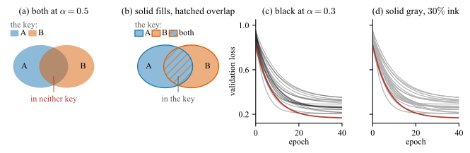
Both failures in Fig. 10.1 come from the same place: an opacity was set for the appearance of a single mark, and Eq. (10.1) was then applied to the places where the marks meet. Both fixes are the panel beside the failure, and they are the same fix: give the distinction to a channel that does not composite.

(image)

Figure 10.1: Two ways an opacity setting says something the figure did not intend. (a) Two class regions at \(\alpha = 0.5\). The intersection renders as a third color that is in neither of them. (b) The same two regions with no opacity anywhere: both classes filled solid and outlined in their own key color, and the area they share carrying one fill under the other class color as a hatch, bounded by one arc of each outline. The page holds only the two colors the key names, the key names the shared area as well, and the draw order changes nothing. (c) and (d) Twenty runs behind the one under discussion: black at \(\alpha = 0.3\) composites over white to exactly the \(30\%\) ink gray of (d), so a lone curve is identical in the two panels and every difference between them is a crossing. Where the runs converge, up to \(7\) of them fall within one line width, and that patch carries \(92\%\) ink in (c) against the \(30\%\) of a lone curve, a factor of \(3.1\).

Two categorical colors must never overlap at \(\alpha \). Fig. 10.1(a) is the failure: the intersection of a blue region and an orange one is a third color, present in the figure and in neither key, and by Eq. (10.1) which of the two possible mixtures it is depends on the order the two were drawn in. The legend is no help. The remedy is to keep the classes in channels that cannot mix. Fig. 10.1(b) fills both classes solid, outlines each in its own key color so the shared area has a boundary of its own, and hatches that area in the other class color: both class colors reach the page exactly as the key shows them, the shared area is visible without being a third color, and it is a third entry in the key rather than something the reader has to decode. Separate panels, or a single hue where the darkness means only “more”, do the same job.

Transparency changes the color

By Eq. (10.1) the color on the page is not the color in the palette, and it changes again if the panel is later given a background: the same mark at \(\alpha = 0.5\) is one color over white and another over a gray panel. So the gray print and the color vision deficiency checks of Sec. 5.5 have to be run on the rendered figure rather than on the palette it was specified from, and a colormap loses its perceptual uniformity as soon as an opacity is applied to it.

For de-emphasis, use a light solid color rather than \(\alpha \). Drawing the context series in black at low opacity, is not the same as drawing them light: the crossings accumulate by Eq. (10.2) and darken wherever the series happen to bunch. Fig. 10.1(c) and (d) are the same twenty runs de-emphasized both ways, matched so that a lone curve renders identically in the two panels. The alpha panel grows a dark bar exactly where the runs converge, which competes with the highlighted curve for the attention the highlight was supposed to own, and which reports a bunching that no key on the page quantifies.

10.2 Accumulation

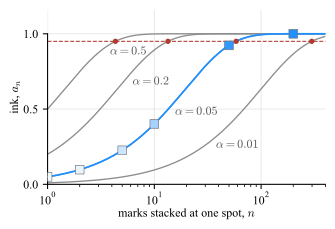
Used deliberately, the same accumulation is the point: a dense scatter stops being a silhouette and becomes a density display. That makes \(\alpha \) a magnitude channel, sixth in the ranking of Sec. 6. It is also a channel that runs out, as Fig. 10.2 shows.

(image)

Figure 10.2: The ink \(a_n\) of Eq. (10.2) against the number of marks stacked at one spot, for four opacities. The squares on the \(\alpha = 0.05\) curve are filled with the color the page actually renders at \(n = 1\), \(2\), \(5\), \(10\), \(50\) and \(200\), so the curve can be checked against its own ink. Past the dashed level at \(0.95\), marked on each curve by a dot, a further mark changes nothing the reader can see.

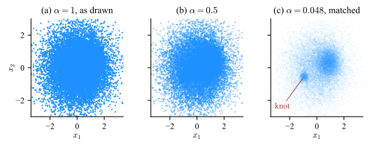
Set \(\alpha \) from the overlap, not by taste. Eq. (10.2) saturates, and quickly. Ink reaches \(95\%\) of full at \(n^{\ast } = \ln (0.05) / \ln (1-\alpha ) \approx 3/\alpha \), which is \(4.3\) marks at \(\alpha = 0.5\) and \(58.4\) at \(\alpha = 0.05\). Past that count the channel is exhausted and the picture is a silhouette again, which is why Fig. 10.3(b) is barely an improvement on Fig. 10.3(a). The working rule is

\begin{equation} \alpha \approx \frac {1}{n_{\mathrm {typ}}} , \label {eq-plot-alpha-rule} \end{equation}

where \(n_{\mathrm {typ}}\) is the number of marks that typically share one marker footprint, which is a property of the data and the marker size and can be counted rather than guessed. It puts the typical spot at \(1 - e^{-1} = 0.63\) of full ink, in the middle of the channel with room above it for the crowded spots and below it for the sparse ones.

(image)

Figure 10.3: Twenty thousand points from a broad cloud holding a dense core and a small tight knot, drawn three ways on identical axes with identical \(1.6\) pt markers. (a) At \(\alpha = 1\), \(88.0\%\) of the points land on ink that is already full, so the panel reports the outline of the cloud and the accident of draw order, and neither the core nor the knot survives. (b) At \(\alpha = 0.5\), \(54.0\%\) of them still do, because ink is \(0.99\) of full by the seventh mark: halving the opacity does not halve the problem. (c) At \(\alpha = 0.048\), which is \(1/n_{\mathrm {typ}}\) for a measured typical overlap of \(n_{\mathrm {typ}} = 21\) marks per marker footprint, the core and the knot both appear. The price is that a lone point now carries \(4.8\%\) ink, near the edge of what can be seen at all.

The same choice hides the isolated point. An \(\alpha \) small enough to resolve a crowd renders a lone mark at \(\alpha \) of full ink and nothing more, \(4.8\%\) in Fig. 10.3(c), so the outlier that a scatter is often drawn to find is the first thing the setting removes. Where both matter, the two populations are two layers: the crowd at low \(\alpha \), and the points that are alone drawn separately at full strength.

Transparency is a magnitude channel without a key

A scatter at \(\alpha < 1\) encodes count as darkness, so it falls under the rule of Sec. 6.4: every magnitude channel needs a zero and a key. It has neither, and Eq. (10.2) is not linear in the count either, so the darkness cannot be read back even in principle. Use it to reveal that structure exists, never to report how much of it there is.

PDF file size

A transparent mark forces a transparency group into the PDFT. The twenty thousand markers of each panel of Fig. 10.3 make a \(0.9\) MB file that is slow to open and slower to print. Rasterizing the dense layer alone, keeps the axes and every label vector while the cloud becomes an image at the export resolution, and brings the same figure to \(205\) kB.