Plotting

\(\newcommand{\footnotename}{footnote}\) \(\def \LWRfootnote {1}\) \(\newcommand {\footnote }[2][\LWRfootnote ]{{}^{\mathrm {#1}}}\) \(\newcommand {\footnotemark }[1][\LWRfootnote ]{{}^{\mathrm {#1}}}\) \(\let \LWRorighspace \hspace \) \(\renewcommand {\hspace }{\ifstar \LWRorighspace \LWRorighspace }\) \(\newcommand {\TextOrMath }[2]{#2}\) \(\newcommand {\mathnormal }[1]{{#1}}\) \(\newcommand \ensuremath [1]{#1}\) \(\newcommand {\LWRframebox }[2][]{\fbox {#2}} \newcommand {\framebox }[1][]{\LWRframebox } \) \(\newcommand {\setlength }[2]{}\) \(\newcommand {\addtolength }[2]{}\) \(\newcommand {\setcounter }[2]{}\) \(\newcommand {\addtocounter }[2]{}\) \(\newcommand {\arabic }[1]{}\) \(\newcommand {\number }[1]{}\) \(\newcommand {\noalign }[1]{\text {#1}\notag \\}\) \(\newcommand {\cline }[1]{}\) \(\newcommand {\directlua }[1]{\text {(directlua)}}\) \(\newcommand {\luatexdirectlua }[1]{\text {(directlua)}}\) \(\newcommand {\protect }{}\) \(\def \LWRabsorbnumber #1 {}\) \(\def \LWRabsorbquotenumber "#1 {}\) \(\newcommand {\LWRabsorboption }[1][]{}\) \(\newcommand {\LWRabsorbtwooptions }[1][]{\LWRabsorboption }\) \(\def \mathchar {\ifnextchar "\LWRabsorbquotenumber \LWRabsorbnumber }\) \(\def \mathcode #1={\mathchar }\) \(\let \delcode \mathcode \) \(\let \delimiter \mathchar \) \(\def \oe {\unicode {x0153}}\) \(\def \OE {\unicode {x0152}}\) \(\def \ae {\unicode {x00E6}}\) \(\def \AE {\unicode {x00C6}}\) \(\def \aa {\unicode {x00E5}}\) \(\def \AA {\unicode {x00C5}}\) \(\def \o {\unicode {x00F8}}\) \(\def \O {\unicode {x00D8}}\) \(\def \l {\unicode {x0142}}\) \(\def \L {\unicode {x0141}}\) \(\def \ss {\unicode {x00DF}}\) \(\def \SS {\unicode {x1E9E}}\) \(\def \dag {\unicode {x2020}}\) \(\def \ddag {\unicode {x2021}}\) \(\def \P {\unicode {x00B6}}\) \(\def \copyright {\unicode {x00A9}}\) \(\def \pounds {\unicode {x00A3}}\) \(\let \LWRref \ref \) \(\renewcommand {\ref }{\ifstar \LWRref \LWRref }\) \( \newcommand {\multicolumn }[3]{#3}\) \(\require {textcomp}\) \( \newcommand {\abs }[1]{\lvert #1\rvert } \) \( \DeclareMathOperator {\sign }{sign} \) \(\newcommand {\intertext }[1]{\text {#1}\notag \\}\) \(\let \Hat \hat \) \(\let \Check \check \) \(\let \Tilde \tilde \) \(\let \Acute \acute \) \(\let \Grave \grave \) \(\let \Dot \dot \) \(\let \Ddot \ddot \) \(\let \Breve \breve \) \(\let \Bar \bar \) \(\let \Vec \vec \) \(\newcommand {\bm }[1]{\boldsymbol {#1}}\) \(\require {physics}\) \(\newcommand {\LWRphystrig }[2]{\ifblank {#1}{\textrm {#2}}{\textrm {#2}^{#1}}}\) \(\renewcommand {\sin }[1][]{\LWRphystrig {#1}{sin}}\) \(\renewcommand {\sinh }[1][]{\LWRphystrig {#1}{sinh}}\) \(\renewcommand {\arcsin }[1][]{\LWRphystrig {#1}{arcsin}}\) \(\renewcommand {\asin }[1][]{\LWRphystrig {#1}{asin}}\) \(\renewcommand {\cos }[1][]{\LWRphystrig {#1}{cos}}\) \(\renewcommand {\cosh }[1][]{\LWRphystrig {#1}{cosh}}\) \(\renewcommand {\arccos }[1][]{\LWRphystrig {#1}{arcos}}\) \(\renewcommand {\acos }[1][]{\LWRphystrig {#1}{acos}}\) \(\renewcommand {\tan }[1][]{\LWRphystrig {#1}{tan}}\) \(\renewcommand {\tanh }[1][]{\LWRphystrig {#1}{tanh}}\) \(\renewcommand {\arctan }[1][]{\LWRphystrig {#1}{arctan}}\) \(\renewcommand {\atan }[1][]{\LWRphystrig {#1}{atan}}\) \(\renewcommand {\csc }[1][]{\LWRphystrig {#1}{csc}}\) \(\renewcommand {\csch }[1][]{\LWRphystrig {#1}{csch}}\) \(\renewcommand {\arccsc }[1][]{\LWRphystrig {#1}{arccsc}}\) \(\renewcommand {\acsc }[1][]{\LWRphystrig {#1}{acsc}}\) \(\renewcommand {\sec }[1][]{\LWRphystrig {#1}{sec}}\) \(\renewcommand {\sech }[1][]{\LWRphystrig {#1}{sech}}\) \(\renewcommand {\arcsec }[1][]{\LWRphystrig {#1}{arcsec}}\) \(\renewcommand {\asec }[1][]{\LWRphystrig {#1}{asec}}\) \(\renewcommand {\cot }[1][]{\LWRphystrig {#1}{cot}}\) \(\renewcommand {\coth }[1][]{\LWRphystrig {#1}{coth}}\) \(\renewcommand {\arccot }[1][]{\LWRphystrig {#1}{arccot}}\) \(\renewcommand {\acot }[1][]{\LWRphystrig {#1}{acot}}\) \(\require {cancel}\) \(\newcommand {\underuparrow }[1]{{\underset {\uparrow }{#1}}}\) \(\DeclareMathOperator *{\argmax }{argmax}\) \(\DeclareMathOperator *{\argmin }{arg\,min}\) \(\def \E [#1]{\mathbb {E}\!\left [ #1 \right ]}\) \(\def \Var [#1]{\operatorname {Var}\!\left [ #1 \right ]}\) \(\def \Cov [#1]{\operatorname {Cov}\!\left [ #1 \right ]}\) \(\newcommand {\floor }[1]{\lfloor #1 \rfloor }\) \(\newcommand {\DTFTH }{ H \brk 1{e^{j\omega }}}\) \(\newcommand {\DTFTX }{ X\brk 1{e^{j\omega }}}\) \(\newcommand {\DFTtr }[1]{\mathrm {DFT}\left \{#1\right \}}\) \(\newcommand {\DTFTtr }[1]{\mathrm {DTFT}\left \{#1\right \}}\) \(\newcommand {\DTFTtrI }[1]{\mathrm {DTFT^{-1}}\left \{#1\right \}}\) \(\newcommand {\Ftr }[1]{ \mathcal {F}\left \{#1\right \}}\) \(\newcommand {\FtrI }[1]{ \mathcal {F}^{-1}\left \{#1\right \}}\) \(\newcommand {\Zover }{\overset {\mathscr Z}{\Longleftrightarrow }}\) \(\renewcommand {\real }{\mathbb {R}}\) \(\newcommand {\ba }{\mathbf {a}}\) \(\newcommand {\bb }{\mathbf {b}}\) \(\newcommand {\bc }{\mathbf {c}}\) \(\newcommand {\bd }{\mathbf {d}}\) \(\newcommand {\be }{\mathbf {e}}\) \(\newcommand {\bf }{\mathbf {f}}\) \(\newcommand {\bg }{\mathbf {g}}\) \(\newcommand {\bh }{\mathbf {h}}\) \(\newcommand {\bi }{\mathbf {i}}\) \(\newcommand {\bn }{\mathbf {n}}\) \(\newcommand {\bo }{\mathbf {o}}\) \(\newcommand {\bp }{\mathbf {p}}\) \(\newcommand {\bq }{\mathbf {q}}\) \(\newcommand {\br }{\mathbf {r}}\) \(\newcommand {\bs }{\mathbf {s}}\) \(\newcommand {\bt }{\mathbf {t}}\) \(\newcommand {\bu }{\mathbf {u}}\) \(\newcommand {\bv }{\mathbf {v}}\) \(\newcommand {\bw }{\mathbf {w}}\) \(\newcommand {\bx }{\mathbf {x}}\) \(\newcommand {\bxx }{\mathbf {xx}}\) \(\newcommand {\bxy }{\mathbf {xy}}\) \(\newcommand {\by }{\mathbf {y}}\) \(\newcommand {\byx }{\mathbf {yx}}\) \(\newcommand {\byy }{\mathbf {yy}}\) \(\newcommand {\bz }{\mathbf {z}}\) \(\newcommand {\bA }{\mathbf {A}}\) \(\newcommand {\bB }{\mathbf {B}}\) \(\newcommand {\bC }{\mathbf {C}}\) \(\newcommand {\bD }{\mathbf {D}}\) \(\newcommand {\bH }{\mathbf {H}}\) \(\newcommand {\bI }{\mathbf {I}}\) \(\newcommand {\bK }{\mathbf {K}}\) \(\newcommand {\bM }{\mathbf {M}}\) \(\newcommand {\bP }{\mathbf {P}}\) \(\newcommand {\bQ }{\mathbf {Q}}\) \(\newcommand {\bR }{\mathbf {R}}\) \(\newcommand {\bS }{\mathbf {S}}\) \(\newcommand {\bU }{\mathbf {U}}\) \(\newcommand {\bW }{\mathbf {W}}\) \(\newcommand {\bX }{\mathbf {X}}\) \(\newcommand {\bY }{\mathbf {Y}}\) \(\newcommand {\bZ }{\mathbf {Z}}\) \(\newcommand {\balpha }{\bm {\alpha }}\) \(\newcommand {\bth }{{\bm {\theta }}}\) \(\newcommand {\bepsilon }{{\bm {\epsilon }}}\) \(\newcommand {\bmu }{{\bm {\mu }}}\) \(\newcommand {\bgamma }{{\bm {\gamma }}}\) \(\newcommand {\bphi }{\bm {\phi }}\) \(\newcommand {\bOne }{\mathbf {1}}\) \(\newcommand {\bZero }{\mathbf {0}}\) \(\newcommand {\indFunc }{\mathbb {1}}\) \(\newcommand {\btx }{\tilde {\bx }}\) \(\newcommand {\loss }{\mathcal {L}}\) \(\newcommand {\score }{\mathcal {S}}\) \(\newcommand {\SSE }{\mathrm {SSE}}\) \(\newcommand {\SST }{\mathrm {SST}}\) \(\newcommand {\SSR }{\mathrm {SSR}}\) \(\newcommand {\MSE }{\mathrm {MSE}}\) \(\newcommand {\RMSE }{\mathrm {RMSE}}\) \(\newcommand {\toprule }[1][]{\hline }\) \(\let \midrule \toprule \) \(\let \bottomrule \toprule \) \(\def \LWRbooktabscmidruleparen (#1)#2{}\) \(\newcommand {\LWRbooktabscmidrulenoparen }[1]{}\) \(\newcommand {\cmidrule }[1][]{\ifnextchar (\LWRbooktabscmidruleparen \LWRbooktabscmidrulenoparen }\) \(\newcommand {\morecmidrules }{}\) \(\newcommand {\specialrule }[3]{\hline }\) \(\newcommand {\addlinespace }[1][]{}\) \(\newcommand {\LWRsubmultirow }[2][]{#2}\) \(\newcommand {\LWRmultirow }[2][]{\LWRsubmultirow }\) \(\newcommand {\multirow }[2][]{\LWRmultirow }\) \(\newcommand {\mrowcell }{}\) \(\newcommand {\mcolrowcell }{}\) \(\newcommand {\STneed }[1]{}\) \(\newcommand {\tcbset }[1]{}\) \(\newcommand {\tcbsetforeverylayer }[1]{}\) \(\newcommand {\tcbox }[2][]{\boxed {\text {#2}}}\) \(\newcommand {\tcboxfit }[2][]{\boxed {#2}}\) \(\newcommand {\tcblower }{}\) \(\newcommand {\tcbline }{}\) \(\newcommand {\tcbtitle }{}\) \(\newcommand {\tcbsubtitle [2][]{\mathrm {#2}}}\) \(\newcommand {\tcboxmath }[2][]{\boxed {#2}}\) \(\newcommand {\tcbhighmath }[2][]{\boxed {#2}}\) \(\require {colortbl}\) \(\let \LWRorigcolumncolor \columncolor \) \(\renewcommand {\columncolor }[2][named]{\LWRorigcolumncolor [#1]{#2}\LWRabsorbtwooptions }\) \(\let \LWRorigrowcolor \rowcolor \) \(\renewcommand {\rowcolor }[2][named]{\LWRorigrowcolor [#1]{#2}\LWRabsorbtwooptions }\) \(\let \LWRorigcellcolor \cellcolor \) \(\renewcommand {\cellcolor }[2][named]{\LWRorigcellcolor [#1]{#2}\LWRabsorbtwooptions }\) \(\newcommand {\tothe }[1]{^{#1}}\) \(\newcommand {\raiseto }[2]{{#2}^{#1}}\) \(\newcommand {\LWRsiunitxEND }{}\) \(\def \LWRsiunitxang #1;#2;#3;#4\LWRsiunitxEND {\ifblank {#1}{}{\num {#1}\degree }\ifblank {#2}{}{\num {#2}^{\unicode {x2032}}}\ifblank {#3}{}{\num {#3}^{\unicode {x2033}}}}\) \(\newcommand {\ang }[2][]{\LWRsiunitxang #2;;;\LWRsiunitxEND }\) \(\def \LWRsiunitxdistribunit {}\) \(\newcommand {\LWRsiunitxENDTWO }{}\) \(\def \LWRsiunitxprintdecimalsubtwo #1,#2,#3\LWRsiunitxENDTWO {\ifblank {#1}{0}{\mathrm {#1}}\ifblank {#2}{}{{\LWRsiunitxdecimal }\mathrm {#2}}}\) \(\def \LWRsiunitxprintdecimalsub #1.#2.#3\LWRsiunitxEND {\LWRsiunitxprintdecimalsubtwo #1,,\LWRsiunitxENDTWO \ifblank {#2}{}{{\LWRsiunitxdecimal }\LWRsiunitxprintdecimalsubtwo #2,,\LWRsiunitxENDTWO }}\) \(\newcommand {\LWRsiunitxprintdecimal }[1]{\LWRsiunitxprintdecimalsub #1...\LWRsiunitxEND }\) \(\def \LWRsiunitxnumplus #1+#2+#3\LWRsiunitxEND {\ifblank {#2}{\LWRsiunitxprintdecimal {#1}}{\ifblank {#1}{\LWRsiunitxprintdecimal {#2}}{\LWRsiunitxprintdecimal {#1}\unicode {x02B}\LWRsiunitxprintdecimal {#2}}}\LWRsiunitxdistribunit }\) \(\def \LWRsiunitxnumminus #1-#2-#3\LWRsiunitxEND {\ifblank {#2}{\LWRsiunitxnumplus #1+++\LWRsiunitxEND }{\ifblank {#1}{}{\LWRsiunitxprintdecimal {#1}}\unicode {x02212}\LWRsiunitxprintdecimal {#2}\LWRsiunitxdistribunit }}\) \(\def \LWRsiunitxnumpmmacro #1\pm #2\pm #3\LWRsiunitxEND {\ifblank {#2}{\LWRsiunitxnumminus #1---\LWRsiunitxEND }{\LWRsiunitxprintdecimal {#1}\unicode {x0B1}\LWRsiunitxprintdecimal {#2}\LWRsiunitxdistribunit }}\) \(\def \LWRsiunitxnumpm #1+-#2+-#3\LWRsiunitxEND {\ifblank {#2}{\LWRsiunitxnumpmmacro #1\pm \pm \pm \LWRsiunitxEND }{\LWRsiunitxprintdecimal {#1}\unicode {x0B1}\LWRsiunitxprintdecimal {#2}\LWRsiunitxdistribunit }}\) \(\newcommand {\LWRsiunitxnumscientific }[2]{\ifblank {#1}{}{\ifstrequal {#1}{-}{-}{\LWRsiunitxprintdecimal {#1}\times }}10^{\LWRsiunitxprintdecimal {#2}}\LWRsiunitxdistribunit }\) \(\def \LWRsiunitxnumD #1D#2D#3\LWRsiunitxEND {\ifblank {#2}{\LWRsiunitxnumpm #1+-+-\LWRsiunitxEND }{\mathrm {\LWRsiunitxnumscientific {#1}{#2}}}}\) \(\def \LWRsiunitxnumd #1d#2d#3\LWRsiunitxEND {\ifblank {#2}{\LWRsiunitxnumD #1DDD\LWRsiunitxEND }{\mathrm {\LWRsiunitxnumscientific {#1}{#2}}}}\) \(\def \LWRsiunitxnumE #1E#2E#3\LWRsiunitxEND {\ifblank {#2}{\LWRsiunitxnumd #1ddd\LWRsiunitxEND }{\mathrm {\LWRsiunitxnumscientific {#1}{#2}}}}\) \(\def \LWRsiunitxnume #1e#2e#3\LWRsiunitxEND {\ifblank {#2}{\LWRsiunitxnumE #1EEE\LWRsiunitxEND }{\mathrm {\LWRsiunitxnumscientific {#1}{#2}}}}\) \(\def \LWRsiunitxnumx #1x#2x#3x#4\LWRsiunitxEND {\ifblank {#2}{\LWRsiunitxnume #1eee\LWRsiunitxEND }{\ifblank {#3}{\LWRsiunitxnume #1eee\LWRsiunitxEND \times \LWRsiunitxnume #2eee\LWRsiunitxEND }{\LWRsiunitxnume #1eee\LWRsiunitxEND \times \LWRsiunitxnume #2eee\LWRsiunitxEND \times \LWRsiunitxnume #3eee\LWRsiunitxEND }}}\) \(\newcommand {\num }[2][]{\LWRsiunitxnumx #2xxxxx\LWRsiunitxEND }\) \(\newcommand {\si }[2][]{\mathrm {\gsubstitute {#2}{~}{\,}}}\) \(\def \LWRsiunitxSIopt #1[#2]#3{\def \LWRsiunitxdistribunit {\,\si {#3}}{#2}\num {#1}\def \LWRsiunitxdistribunit {}}\) \(\newcommand {\LWRsiunitxSI }[2]{\def \LWRsiunitxdistribunit {\,\si {#2}}\num {#1}\def \LWRsiunitxdistribunit {}}\) \(\newcommand {\SI }[2][]{\ifnextchar [{\LWRsiunitxSIopt {#2}}{\LWRsiunitxSI {#2}}}\) \(\newcommand {\numlist }[2][]{\text {#2}}\) \(\newcommand {\numrange }[3][]{\num {#2}\ \LWRsiunitxrangephrase \ \num {#3}}\) \(\newcommand {\SIlist }[3][]{\text {#2}\,\si {#3}}\) \(\newcommand {\SIrange }[4][]{\num {#2}\,#4\ \LWRsiunitxrangephrase \ \num {#3}\,#4}\) \(\newcommand {\tablenum }[2][]{\mathrm {#2}}\) \(\newcommand {\ampere }{\mathrm {A}}\) \(\newcommand {\candela }{\mathrm {cd}}\) \(\newcommand {\kelvin }{\mathrm {K}}\) \(\newcommand {\kilogram }{\mathrm {kg}}\) \(\newcommand {\metre }{\mathrm {m}}\) \(\newcommand {\mole }{\mathrm {mol}}\) \(\newcommand {\second }{\mathrm {s}}\) \(\newcommand {\becquerel }{\mathrm {Bq}}\) \(\newcommand {\degreeCelsius }{\unicode {x2103}}\) \(\newcommand {\coulomb }{\mathrm {C}}\) \(\newcommand {\farad }{\mathrm {F}}\) \(\newcommand {\gray }{\mathrm {Gy}}\) \(\newcommand {\hertz }{\mathrm {Hz}}\) \(\newcommand {\henry }{\mathrm {H}}\) \(\newcommand {\joule }{\mathrm {J}}\) \(\newcommand {\katal }{\mathrm {kat}}\) \(\newcommand {\lumen }{\mathrm {lm}}\) \(\newcommand {\lux }{\mathrm {lx}}\) \(\newcommand {\newton }{\mathrm {N}}\) \(\newcommand {\ohm }{\mathrm {\Omega }}\) \(\newcommand {\pascal }{\mathrm {Pa}}\) \(\newcommand {\radian }{\mathrm {rad}}\) \(\newcommand {\siemens }{\mathrm {S}}\) \(\newcommand {\sievert }{\mathrm {Sv}}\) \(\newcommand {\steradian }{\mathrm {sr}}\) \(\newcommand {\tesla }{\mathrm {T}}\) \(\newcommand {\volt }{\mathrm {V}}\) \(\newcommand {\watt }{\mathrm {W}}\) \(\newcommand {\weber }{\mathrm {Wb}}\) \(\newcommand {\day }{\mathrm {d}}\) \(\newcommand {\degree }{\mathrm {^\circ }}\) \(\newcommand {\hectare }{\mathrm {ha}}\) \(\newcommand {\hour }{\mathrm {h}}\) \(\newcommand {\litre }{\mathrm {l}}\) \(\newcommand {\liter }{\mathrm {L}}\) \(\newcommand {\arcminute }{^\prime }\) \(\newcommand {\minute }{\mathrm {min}}\) \(\newcommand {\arcsecond }{^{\prime \prime }}\) \(\newcommand {\tonne }{\mathrm {t}}\) \(\newcommand {\astronomicalunit }{au}\) \(\newcommand {\atomicmassunit }{u}\) \(\newcommand {\bohr }{\mathit {a}_0}\) \(\newcommand {\clight }{\mathit {c}_0}\) \(\newcommand {\dalton }{\mathrm {D}_\mathrm {a}}\) \(\newcommand {\electronmass }{\mathit {m}_{\mathrm {e}}}\) \(\newcommand {\electronvolt }{\mathrm {eV}}\) \(\newcommand {\elementarycharge }{\mathit {e}}\) \(\newcommand {\hartree }{\mathit {E}_{\mathrm {h}}}\) \(\newcommand {\planckbar }{\mathit {\unicode {x210F}}}\) \(\newcommand {\angstrom }{\mathrm {\unicode {x212B}}}\) \(\let \LWRorigbar \bar \) \(\newcommand {\bar }{\mathrm {bar}}\) \(\newcommand {\barn }{\mathrm {b}}\) \(\newcommand {\bel }{\mathrm {B}}\) \(\newcommand {\decibel }{\mathrm {dB}}\) \(\newcommand {\knot }{\mathrm {kn}}\) \(\newcommand {\mmHg }{\mathrm {mmHg}}\) \(\newcommand {\nauticalmile }{\mathrm {M}}\) \(\newcommand {\neper }{\mathrm {Np}}\) \(\newcommand {\yocto }{\mathrm {y}}\) \(\newcommand {\zepto }{\mathrm {z}}\) \(\newcommand {\atto }{\mathrm {a}}\) \(\newcommand {\femto }{\mathrm {f}}\) \(\newcommand {\pico }{\mathrm {p}}\) \(\newcommand {\nano }{\mathrm {n}}\) \(\newcommand {\micro }{\mathrm {\unicode {x00B5}}}\) \(\newcommand {\milli }{\mathrm {m}}\) \(\newcommand {\centi }{\mathrm {c}}\) \(\newcommand {\deci }{\mathrm {d}}\) \(\newcommand {\deca }{\mathrm {da}}\) \(\newcommand {\hecto }{\mathrm {h}}\) \(\newcommand {\kilo }{\mathrm {k}}\) \(\newcommand {\mega }{\mathrm {M}}\) \(\newcommand {\giga }{\mathrm {G}}\) \(\newcommand {\tera }{\mathrm {T}}\) \(\newcommand {\peta }{\mathrm {P}}\) \(\newcommand {\exa }{\mathrm {E}}\) \(\newcommand {\zetta }{\mathrm {Z}}\) \(\newcommand {\yotta }{\mathrm {Y}}\) \(\newcommand {\percent }{\mathrm {\%}}\) \(\newcommand {\meter }{\mathrm {m}}\) \(\newcommand {\metre }{\mathrm {m}}\) \(\newcommand {\gram }{\mathrm {g}}\) \(\newcommand {\kg }{\kilo \gram }\) \(\newcommand {\of }[1]{_{\mathrm {#1}}}\) \(\newcommand {\squared }{^2}\) \(\newcommand {\square }[1]{\mathrm {#1}^2}\) \(\newcommand {\cubed }{^3}\) \(\newcommand {\cubic }[1]{\mathrm {#1}^3}\) \(\newcommand {\per }{\,\mathrm {/}}\) \(\newcommand {\celsius }{\unicode {x2103}}\) \(\newcommand {\fg }{\femto \gram }\) \(\newcommand {\pg }{\pico \gram }\) \(\newcommand {\ng }{\nano \gram }\) \(\newcommand {\ug }{\micro \gram }\) \(\newcommand {\mg }{\milli \gram }\) \(\newcommand {\g }{\gram }\) \(\newcommand {\kg }{\kilo \gram }\) \(\newcommand {\amu }{\mathrm {u}}\) \(\newcommand {\pm }{\pico \metre }\) \(\newcommand {\nm }{\nano \metre }\) \(\newcommand {\um }{\micro \metre }\) \(\newcommand {\mm }{\milli \metre }\) \(\newcommand {\cm }{\centi \metre }\) \(\newcommand {\dm }{\deci \metre }\) \(\newcommand {\m }{\metre }\) \(\newcommand {\km }{\kilo \metre }\) \(\newcommand {\as }{\atto \second }\) \(\newcommand {\fs }{\femto \second }\) \(\newcommand {\ps }{\pico \second }\) \(\newcommand {\ns }{\nano \second }\) \(\newcommand {\us }{\micro \second }\) \(\newcommand {\ms }{\milli \second }\) \(\newcommand {\s }{\second }\) \(\newcommand {\fmol }{\femto \mol }\) \(\newcommand {\pmol }{\pico \mol }\) \(\newcommand {\nmol }{\nano \mol }\) \(\newcommand {\umol }{\micro \mol }\) \(\newcommand {\mmol }{\milli \mol }\) \(\newcommand {\mol }{\mol }\) \(\newcommand {\kmol }{\kilo \mol }\) \(\newcommand {\pA }{\pico \ampere }\) \(\newcommand {\nA }{\nano \ampere }\) \(\newcommand {\uA }{\micro \ampere }\) \(\newcommand {\mA }{\milli \ampere }\) \(\newcommand {\A }{\ampere }\) \(\newcommand {\kA }{\kilo \ampere }\) \(\newcommand {\ul }{\micro \litre }\) \(\newcommand {\ml }{\milli \litre }\) \(\newcommand {\l }{\litre }\) \(\newcommand {\hl }{\hecto \litre }\) \(\newcommand {\uL }{\micro \liter }\) \(\newcommand {\mL }{\milli \liter }\) \(\newcommand {\L }{\liter }\) \(\newcommand {\hL }{\hecto \liter }\) \(\newcommand {\mHz }{\milli \hertz }\) \(\newcommand {\Hz }{\hertz }\) \(\newcommand {\kHz }{\kilo \hertz }\) \(\newcommand {\MHz }{\mega \hertz }\) \(\newcommand {\GHz }{\giga \hertz }\) \(\newcommand {\THz }{\tera \hertz }\) \(\newcommand {\mN }{\milli \newton }\) \(\newcommand {\N }{\newton }\) \(\newcommand {\kN }{\kilo \newton }\) \(\newcommand {\MN }{\mega \newton }\) \(\newcommand {\Pa }{\pascal }\) \(\newcommand {\kPa }{\kilo \pascal }\) \(\newcommand {\MPa }{\mega \pascal }\) \(\newcommand {\GPa }{\giga \pascal }\) \(\newcommand {\mohm }{\milli \ohm }\) \(\newcommand {\kohm }{\kilo \ohm }\) \(\newcommand {\Mohm }{\mega \ohm }\) \(\newcommand {\pV }{\pico \volt }\) \(\newcommand {\nV }{\nano \volt }\) \(\newcommand {\uV }{\micro \volt }\) \(\newcommand {\mV }{\milli \volt }\) \(\newcommand {\V }{\volt }\) \(\newcommand {\kV }{\kilo \volt }\) \(\newcommand {\W }{\watt }\) \(\newcommand {\uW }{\micro \watt }\) \(\newcommand {\mW }{\milli \watt }\) \(\newcommand {\kW }{\kilo \watt }\) \(\newcommand {\MW }{\mega \watt }\) \(\newcommand {\GW }{\giga \watt }\) \(\newcommand {\J }{\joule }\) \(\newcommand {\uJ }{\micro \joule }\) \(\newcommand {\mJ }{\milli \joule }\) \(\newcommand {\kJ }{\kilo \joule }\) \(\newcommand {\eV }{\electronvolt }\) \(\newcommand {\meV }{\milli \electronvolt }\) \(\newcommand {\keV }{\kilo \electronvolt }\) \(\newcommand {\MeV }{\mega \electronvolt }\) \(\newcommand {\GeV }{\giga \electronvolt }\) \(\newcommand {\TeV }{\tera \electronvolt }\) \(\newcommand {\kWh }{\kilo \watt \hour }\) \(\newcommand {\F }{\farad }\) \(\newcommand {\fF }{\femto \farad }\) \(\newcommand {\pF }{\pico \farad }\) \(\newcommand {\K }{\mathrm {K}}\) \(\newcommand {\dB }{\mathrm {dB}}\) \(\newcommand {\kibi }{\mathrm {Ki}}\) \(\newcommand {\mebi }{\mathrm {Mi}}\) \(\newcommand {\gibi }{\mathrm {Gi}}\) \(\newcommand {\tebi }{\mathrm {Ti}}\) \(\newcommand {\pebi }{\mathrm {Pi}}\) \(\newcommand {\exbi }{\mathrm {Ei}}\) \(\newcommand {\zebi }{\mathrm {Zi}}\) \(\newcommand {\yobi }{\mathrm {Yi}}\) \(\let \unit \si \) \(\let \qty \SI \) \(\let \qtylist \SIlist \) \(\let \qtyrange \SIrange \) \(\let \numproduct \num \) \(\let \qtyproduct \SI \) \(\let \complexnum \num \) \(\newcommand {\complexqty }[3][]{(\complexnum {#2})\si {#3}}\) \(\renewcommand {\pm }{\mathbin {\unicode {x00B1}}}\) \(\def \LWRsiunitxrangephrase {\TextOrMath { }{\ }\protect \mbox {to}\TextOrMath { }{\ }}\) \(\def \LWRsiunitxdecimal {.}\)

A Tables

A table is the right display when the reader looks values up by name (Sec. 4.1), and it is subject to the same economy as a figure: every rule, color and digit either helps a reader find and compare numbers or competes with the numbers for attention. Unlike a figure, a table gets no help from the parallel stage of vision (Sec. 4). It is read serially, cell by cell, so its layout decides how long each look-up takes and whether a comparison can be made at all.

Each rule below is shown twice on the same numbers: (a) a counterexample that breaks it and (b) an example that follows it. Most of the tables use one running case, the six classifiers of Fig. 11.1, with illustrative scores, fold-to-fold spreads and training times. Every one of those tables is sorted by its quantity of interest, best first, in both of its panels, so that the two panels differ only in the rule they illustrate: by F1 wherever F1 is shown, and by training time, fastest first, in the one table that shows only time. The exception is Sec. A.7, where the row order is itself the rule under test.

A.1 Table or figure

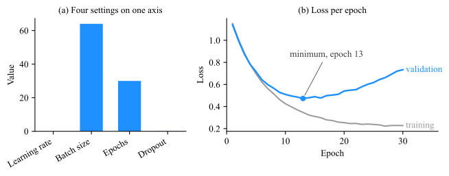
Use a table when the reader needs a few exact values, looked up by name, especially values with different units or values that will be copied elsewhere. Use a figure when the question is about shape: a trend, a minimum, a crossing, a group. The two directions fail differently, so both are shown.

(image)

Figure A.1: (a) Counterexample. Four hyperparameters drawn as bars on one axis. They share no unit and span five orders of magnitude, so the learning rate and the dropout rate vanish, and the two visible bars cannot be read to the exact value that a reader copying the setup needs. (b) Example. Training and validation loss per epoch. The question is where validation stops improving, and the curve answers it at a glance: epoch 13, after which the gap to the training loss only grows.
Table A.1: The same two data sets in the other form. A handful of exact, mixed-unit settings reads best as a table; thirty losses do not.
(a) Counterexample. The losses of Fig. A.1(b), every second epoch. The minimum hides among fifteen similar rows, and the sampling a table forces has moved it: the smallest validation loss here is at epoch 16, not 13.
.
Epoch Training Validation
2 1.009 0.999
4 0.781 0.782
6 0.621 0.643
8 0.515 0.566
10 0.425 0.510
12 0.370 0.486
14 0.323 0.479
16 0.299 0.477
18 0.273 0.504
20 0.254 0.540
22 0.247 0.553
24 0.241 0.601
26 0.234 0.644
28 0.228 0.691
30 0.228 0.733
   
(b) Example. The hyperparameters of Fig. A.1(a). Each value is exact, each carries its own unit, and each is found by name in one step.
.
Hyperparameter Value
Learning rate \(3\times 10^{-4}\)
Batch size 64
Epochs 30
Dropout rate 0.1

One number is not a table

A single value, or two, belongs in the sentence. A table of one row makes the reader leave the text, find the float, and come back for nothing.

A.2 Round to what the data support

A digit is worth printing only if it could change a conclusion. When a score varies by \(0.01\) from one cross-validation fold to the next, its third decimal is noise, and printing six decimals makes the reader parse four digits of noise per cell before reaching the two that matter. Ehrenberg’s working rule is two effective digits, the digits that vary across the column: they are what the eye can hold and compare. Round the spread to one or two significant digits and the value to the same decimal place.

Table A.2: F1 score, mean \(\pm \) standard deviation over five folds. Rounded to the spread, the ranking and its uncertainty read in one pass.
(a) Counterexample. Every digit the software printed.
.
Model F1
Gradient boosting \(0.863127 \pm 0.012185\)
Random forest \(0.829915 \pm 0.012074\)
MLP \(0.801356 \pm 0.023712\)
SVM \(0.790427 \pm 0.019866\)
k-NN \(0.738562 \pm 0.028341\)
Ridge \(0.713184 \pm 0.021507\)
   
(b) Example. The spread to one significant digit, the mean to the same decimal place.
.
Model F1
Gradient boosting \(0.86 \pm 0.01\)
Random forest \(0.83 \pm 0.01\)
MLP \(0.80 \pm 0.02\)
SVM \(0.79 \pm 0.02\)
k-NN \(0.74 \pm 0.03\)
Ridge \(0.71 \pm 0.02\)
A.3 Three horizontal rules, no vertical ones

A table needs three rules: one above the header, one below it, and one at the bottom. Columns are already separated by the white space between them, which the eye groups by proximity (Sec. 9); a vertical rule adds a line the reader has to cross on every comparison along a row. A full grid turns every cell into a box, and the boxes, not the numbers, become the dominant pattern on the page.

Table A.3: The same twelve numbers in a grid and in the three-rule layout. The grid adds nine lines and no information.
(a) Counterexample. Vertical rules, a rule under every row, and a double rule under the header.
.
Model F1 Accuracy Time (s)
Gradient boosting 0.86 0.89 41.2
Random forest 0.83 0.87 8.3
SVM 0.79 0.84 12.6
Ridge 0.71 0.78 0.4
   
(b) Example. Top, middle and bottom rules only; the columns are separated by space.
.
Model F1 Accuracy Time (s)
Gradient boosting 0.86 0.89 41.2
Random forest 0.83 0.87 8.3
SVM 0.79 0.84 12.6
Ridge 0.71 0.78 0.4
A.4 Group with space and short rules

When columns or rows fall into groups, show the grouping with the lightest device that works. A spanning header with a short rule under it (\cmidrule in LaTeX) groups the columns beneath it, and a group label on its own row, set off by a little space, groups the rows. Full-width rules between groups and vertical rules between column blocks do the same job at a much higher ink cost, and they cut the table into boxes that the reader then has to reassemble.

Table A.4: Validation and test scores for three families of models. The grouping is identical in the two versions; only the device that shows it differs.
(a) Counterexample. The column blocks are fenced by vertical rules, the families by full rules, and the family is repeated in a column of its own.
.
Validation Test
Family Model F1 Accuracy F1 Accuracy
Tree ensemble Gradient boosting 0.86 0.89 0.84 0.88
Tree ensemble Random forest 0.83 0.87 0.81 0.86
Neural MLP 0.80 0.85 0.79 0.84
Classical SVM 0.79 0.84 0.78 0.83
Classical k-NN 0.74 0.80 0.72 0.79
Classical Ridge 0.71 0.78 0.70 0.77
(b) Example. Short rules under the spanning headers, and each family named once, on its own row.
.
Validation Test
Model F1 Accuracy F1 Accuracy
Tree ensembles
 Gradient boosting 0.86 0.89 0.84 0.88
 Random forest 0.83 0.87 0.81 0.86
Neural
 MLP 0.80 0.85 0.79 0.84
Classical
 SVM 0.79 0.84 0.78 0.83
 k-NN 0.74 0.80 0.72 0.79
 Ridge 0.71 0.78 0.70 0.77
A.5 Text left, numbers on the decimal point

Text is read from its first letter, so text columns are left-aligned. Numbers are compared by magnitude, and magnitude is carried by the digits to the left of the decimal point, so numbers are aligned on it: with the same number of decimals in a column, the longer number is visibly the larger one, and the column works as a crude bar chart. Centered numbers lose that, because the position of the decimal point wanders from row to row. In LaTeX, the S column of the siunitx package aligns on the decimal point.

Table A.5: Training time of the six models, fastest first. Aligned on the decimal point, each order of magnitude adds one digit of width, and the two slow models stand out by length alone.
(a) Counterexample. Every column centered, with a varying number of decimals.
.
Model Time (s)
k-NN 0.12
Ridge 0.4
Random forest 8.31
SVM 12.6
Gradient boosting 41.2
MLP 95.7
   
(b) Example. Names left-aligned, times aligned on the decimal point with one decimal throughout.
.
Model Time (s)
k-NN 0.1
Ridge 0.4
Random forest 8.3
SVM 12.6
Gradient boosting 41.2
MLP 95.7
A.6 Units in the header, one format per column

A unit or a scale factor that applies to a whole column is stated once, in its header, and every cell of the column then uses the same unit, the same number format and the same number of decimals. Anything else makes the reader convert before comparing: \(86\%\) against \(0.85\), or 1 min 36 s against 41 s. A negative number takes a true minus sign (\(-0.15\)), not a hyphen (-0.15), which is shorter and sits at a different height.

Table A.6: Accuracy, training time, and the F1 gap to the best model. Only the format differs between the two versions.
(a) Counterexample. Units in the cells, three formats for accuracy, four spellings of seconds, and hyphens for minus signs.
.
Model Accuracy Time F1 gap
Gradient boosting 0.89 41 s 0
Random forest 87 % 8.3s -0.03
MLP 85% 1 min 36 s -0.06
SVM .84 12.6 sec -0.07
k-NN 80% 120 ms -0.12
Ridge 0.78 0.4 s -0.15
(b) Example. Units in the headers, one format per column, true minus signs.
.
Model Accuracy Time (s) F1 gap
Gradient boosting 0.89 41.2 \(0.00\)
Random forest 0.87 8.3 \(-0.03\)
MLP 0.85 95.7 \(-0.06\)
SVM 0.84 12.6 \(-0.07\)
k-NN 0.80 0.1 \(-0.12\)
Ridge 0.78 0.4 \(-0.15\)
A.7 Order the rows by what the reader wants

Row order decides which question a table answers, exactly as it did for the chart of Fig. 4.3. A results table is read for ranking, so its rows are sorted by the quantity of interest, and the best and worst models are then the first and last rows. Alphabetical order is the default of most software and serves only a reader who arrives with a name. When the rows have a natural order of their own (time, dose, model size), that order wins over both.

Table A.7: Validation F1 of the six models. Sorted, the ranking is the table; alphabetical, it has to be reconstructed.
(a) Counterexample. Alphabetical order: to find the runner-up the reader compares all six values.
.
Model F1
Gradient boosting 0.86
k-NN 0.74
MLP 0.80
Random forest 0.83
Ridge 0.71
SVM 0.79
   
(b) Example. Sorted by F1, best first: the ranking is read from top to bottom.
.
Model F1
Gradient boosting 0.86
Random forest 0.83
MLP 0.80
SVM 0.79
k-NN 0.74
Ridge 0.71
A.8 Compare down a column

Numbers that are to be compared go in a column, one above the other. Down a column the digits of equal weight sit under each other, the decimal points line up, and the eye runs a short vertical path; along a row, each value is separated from the next by a whole cell and the digits no longer line up. The items being compared, here the models, are therefore the rows, and the measures are the columns. A table with more items than measures is also taller than it is wide, which is the shape a page holds.

Table A.8: The six models on three measures. Transposed, each measure is one column of like numbers.
(a) Counterexample. Models as columns: every comparison between models runs along a row.
.
Gradient boosting Random forest MLP SVM k-NN Ridge
F1 0.86 0.83 0.80 0.79 0.74 0.71
Accuracy 0.89 0.87 0.85 0.84 0.80 0.78
Time (s) 41.2 8.3 95.7 12.6 0.1 0.4
(b) Example. Models as rows: each comparison runs down a column.
.
Model F1 Accuracy Time (s)
Gradient boosting 0.86 0.89 41.2
Random forest 0.83 0.87 8.3
MLP 0.80 0.85 95.7
SVM 0.79 0.84 12.6
k-NN 0.74 0.80 0.1
Ridge 0.71 0.78 0.4
A.9 Emphasize sparingly

Emphasis in a table is the pre-attentive pop-out of Sec. 4 put to work: one bold value in a column is found without a search. That works only while it is rare. Bold on every good value, a second color for another criterion and shading on alternate rows leave nothing standing out, and they add a conjunction search (which values are bold and red?) that the reader cannot do at a glance. Mark the one thing per column the reader is looking for, usually the best value, and push the reference row back in gray rather than forward in color.

Table A.9: The same results, emphasized two ways. With one mark per column, the winner of each measure is found without reading.
(a) Counterexample. Striped rows, every F1 and accuracy at or above \(0.80\) in bold red, every time below \(10\) s in blue.
.
Model F1 Accuracy Time (s)
Gradient boosting 0.86 0.89 41.2
Random forest 0.83 0.87 8.3
MLP 0.80 0.85 95.7
SVM 0.79 0.84 12.6
k-NN 0.74 0.80 0.1
Ridge 0.71 0.78 0.4
   
(b) Example. The best value of each column in bold, the Ridge baseline in gray.
.
Model F1 Accuracy Time (s)
Gradient boosting 0.86 0.89 41.2
Random forest 0.83 0.87 8.3
MLP 0.80 0.85 95.7
SVM 0.79 0.84 12.6
k-NN 0.74 0.80 0.1
Ridge (baseline) 0.71 0.78 0.4
A.10 Shade cells only for one homogeneous quantity

Shading each cell by its value turns a table into a heatmap: the pattern is seen at once, and the exact values stay readable. It is honest only when every shaded cell holds the same quantity on the same scale, as in the relations of Sec. 6.4: a confusion matrix, a correlation matrix, a distance matrix. Shade a results table instead, and the reader applies one reading, darker is more, to columns with different units and different directions. Darker is better for F1 and worse for training time, and nothing in the color says so. The colormap choices of Sec. 5.4 apply unchanged: a sequential map for a quantity with a low and a high end, light enough at the top of the scale that the numbers stay legible.

Table A.10: Shading is read as “darker is more”. On a results table that reading makes the best model and the slowest one look alike; on a confusion matrix it shows the diagonal at once.
(a) Counterexample. One colormap over F1 and training time. The darkest cells are the best F1 and the slowest training, and they look alike.
.
Model F1 Time (s)
Gradient boosting
0.86
41.2
Random forest
0.83
8.3
MLP
0.80
95.7
SVM
0.79
12.6
k-NN
0.74
0.1
Ridge
0.71
0.4
   
(b) Example. The confusion matrix of gradient boosting on three classes, as a percentage of each true class. One quantity, one scale, and the dark diagonal is the pattern.
.
Predicted (%)
True class Normal Fault A Fault B
Normal
90
6
4
Fault A
15
70
15
Fault B
5
10
85
A.11 A caption above the table that states the finding

A table caption goes above the table, because a table is read from the top and the reader should know what to look for before the first row. As with figures (Sec. 12), the caption states what the table shows, not what it contains: the header row already says that the columns are F1 and accuracy.

Table A.11: Placed above and stating the result, a caption tells the reader what to check before the first row is read. The pseudo-captions are set inside the panels, where each version puts them.
(a) Counterexample. A caption below the table that names its contents.
.
Model F1 Accuracy
Gradient boosting 0.86 0.89
Random forest 0.83 0.87
MLP 0.80 0.85

Table 3: Results.

   
(b) Example. A caption above the table that states the result.

Table 3: Gradient boosting leads on both measures, and its F1 margin over the random forest, \(0.03\), is three times the fold-to-fold spread.

.
Model F1 Accuracy
Gradient boosting 0.86 0.89
Random forest 0.83 0.87
MLP 0.80 0.85
Further reading