A chart maps numbers onto a visual channel, and the channels are not interchangeable. Their accuracy has been measured. The ranking is stable, and it is the most useful result in the field:
1. position along a common scale;
2. length;
3. slope and angle;
4. area;
5. volume;
6. shading and color strength;
7. a different color.
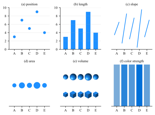
Fig. 6.1 puts one set of five values through the first six of these channels, one panel per entry, from panel (a) for the first to panel (f) for the sixth, so the
ranking can be felt rather than taken on trust. The seventh has no panel here because it has no answer: a set of colors is a set of names, and names do not come in an order, so the ranking cannot be recovered at all. Only the
dark-to-light part of a color can be ranked, which is the subject of Sec. 5.1.
Figure 6.1: Five values, \(A\) to \(E\), encoded six ways, one panel per entry of the ranking above. Rank the categories from smallest to largest in each panel. The answer is \(A < E < C < B < D\) throughout.
Panels (a) and (b) give it up immediately. Panels (c) to (e) take effort and invite errors between the close pair \(B\) and \(C\), and the two size channels differ in how much of the difference survives: \(D\) is three times \(A\), and
its mark has three times the area in (d) and only \(2.1\) times in (e), where the value is a volume, so the radius of the ball and the edge of the cube both follow its cube root. Panel (f) cannot be done reliably at all.
Three consequences follow, and they account for most of the chart-type advice in circulation.
Bar, line and scatter
Bar, line and scatter are the workhorses. They occupy the top of the ranking. There is rarely a reason to reach past them for quantitative data.
6.1 Case Study: Pie and 3D plots
Pie charts encode angle and area
Both sit low in the ranking, which is why comparing two slices of similar size is guesswork, and why a pie with more than three slices cannot be ordered by eye. The same numbers as a sorted bar chart are read exactly, in the same
space.
Three dimensions on a flat page cost accuracy and buy nothing
A 3D bar chart replaces length, which is second in the ranking, with volume under projection, which is fifth, and adds occlusion so that some bars hide others. Adding perspective makes it worse than guesswork: tilting the pie
shrinks the back slices and enlarges the front ones, so the picture is no longer even a faithful rendering of the angles.
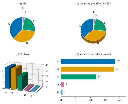
Both paragraphs above can be checked on one set of numbers. Fig. 6.2 takes the five values \(37\), \(36\), \(24\), \(2\) and \(1\) through the four charts a spreadsheet offers
for them. The two largest differ by one part in a hundred, and that difference is the test: every panel contains it, and one panel shows it.
Figure 6.2: Five values, \(A=37\), \(B=36\), \(C=24\), \(D=2\), \(E=1\), drawn four ways. (a) A pie: \(A\) and \(B\) differ by \(3.6^{\circ }\) of arc out of \(360^{\circ }\), so the two cannot be ordered, and the slivers
\(D\) and \(E\) need leaders to be labeled at all. (b) The same pie tilted by \(28^{\circ }\): \(B\) lies at the front and collects the slab wall, so it is drawn with \(1.27\) times the apparent area of \(A\) although it is the smaller
value. (c) The same values as 3D bars: the front bar tops reads between \(7\) and \(11\) units low, which distorts the differences as well as the values. (d) Sorted bars with the values printed: the ranking is immediate and the
numbers are exact.
Panel (d) is not a more careful version of the others, it is a different encoding. It reads the values as length from a common baseline, second in the ranking, while (a) and (b) read them as angle and area, third and fourth, and
(c) reads them as a height that has to be carried across a gap in depth before it meets a scale.
6.2 Case Study: Three variables on a flat page
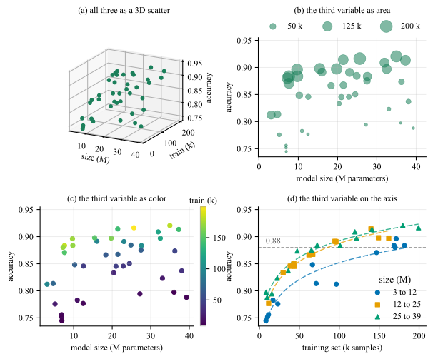
Two variables get the two axes. A third has to go into a channel, and which channel is the whole question, because the ranking above is the answer to it. Fig. 6.3 takes one
record of forty training runs, each with a model size, a training set size and the accuracy it reached, and moves the training set size through four channels, one per panel. The reader is meant to take off the page that model size
stops paying past about ten million parameters and training set size does not, so which of the two is worth the next budget.
Figure 6.3: Three variables. (a) All three as a 3D scatter. (b) The training set as marker area. (c) The training set as color, on viridis with a colorbar. (d) The training set on the horizontal axis, model size as
three bins in color (Okabe-Ito scheme) and marker shape at once.
The four panels are four entries of the ranking, and they come out in its order.
• Panel (a) is not on the ranking at all: a projected point has no depth to decode, which is the argument of Sec. 6.1 moved from
a pie to a scatter.
• Panel (b) reads it as area, fourth.
• Panel (c) reads it as color strength, sixth, which supports more and less and stops there.
• Panel (d) reads the third variable as position on a common scale, first, which is why the number the question turns on is read off an axis instead of estimated.
Note (d) carries model size in two channels at once, color and marker shape.
6.3 Case Study: Radar charts
Radar chart
A radar chart, also called a spider or a web chart, places \(k\) categories at \(k\) equally spaced angles, draws each value as a radius along its own spoke, and joins the ends into a closed polygon. The angle is a
slot rather than a quantity, which is what separates it from a polar plot: there the angle carries a direction, a phase or a time of day, and none of what follows applies.
The form has one honest use and it is narrow: a small number of profiles, measured on axes that genuinely share a scale, read for their shape rather than for their values. Every attribute is scored by the same panel on the same
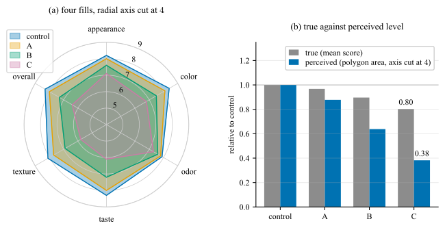
scale, so the radial axis means one thing on every spoke. Fig. 6.4 takes one such record, four samples scored on six attributes, draws it in the form the chart usually takes, and
measures beside it what that form does to the levels.
Figure 6.4: One synthetic sensory record: four samples, six attributes, every attribute scored on the same \(9\)-point scale, drawn as a radar chart and measured against it. (a) All four filled at \(\alpha = 0.35\) on a radial
axis starting at \(4\). The cut removes the inner \(44\,\%\) of every radius and takes the apparent area of sample C; the fills occlude one another in the order they were drawn. (b) The cost of that encoding, as a length: for each
sample, the true level, its mean score relative to the control, beside the level the polygon area of panel (a) makes the reader perceive, both on a zero baseline.
Panel (b) measures what panel (a) costs. The gray bar is what a sample scored, the blue bar is the level its polygon in panel (a) makes the reader perceive. The gap between the two is contributed by the encoding
rather than by the data: nothing on panel (a) discloses that they differ. The gap widens with the drop, from \(0.09\) for sample A to \(0.42\) for sample C, so the chart is least trustworthy exactly where the finding is.
What panel (a) does wrong follows from what the polygon is. Its area on \(k\) equally spaced spokes with radii \(r_1,\dots ,r_k\) is
and two properties of that expression decide how the chart reads.
The area is quadratic in the values. The eye compares the filled shapes and not the radii. Sample C scores \(0.803\) of the control level and its polygon covers \(0.646\) of the control area, which overstates the drop by a
factor of \(1.80\); that comparison is the pair of bars panel (b) draws. That is the exaggeration of a cut bar chart (Sec. 7) in a form no axis label discloses.
The area depends on the order of the spokes. Eq. (6.1) pairs adjacent radii only, so permuting the axes changes it without
changing a number. On this record the effect is small. The ordering is a choice the author makes and the reader cannot see.
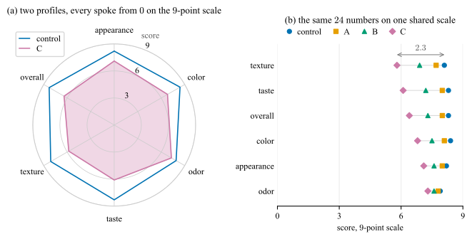
The fix for panel (a) is not a better radar chart. The same \(24\) numbers as a dot plot, one row per attribute and one marker per sample on a shared horizontal scale, drawn in Fig. 6.5(b), put all of them at the top of the ranking of Sec. 6: the largest difference in the record, \(2.3\) points of
texture between the control and sample C, becomes a length rather than a shape. It also settles the comparison the radar chart cannot serve at all. Two attributes of one sample sit on one scale in a dot plot; on a radar chart
they sit in two different directions.
If you draw one
One zero-anchored scale on every spoke, and name it. Two profiles at most, or one per panel as small multiples (Sec. 7.6). Fill one polygon or none. And say what fixes the
axis order, because Eq. (6.1) says the picture depends on it.
Fig. 6.5(a) is that box applied to the record of Fig. 6.4, and panel (b) is the dot plot beside it.
Panel (a) is as good as the form gets, and it is still the weaker of the two. Anchoring the radial axis at zero fixes the baseline and nothing else: by Eq. (6.1) the area stays quadratic in the scores, so sample C keeps \(0.803\) of the control level and \(0.646\) of the area, the same factor of \(1.80\) as before; the
spoke order still moves the picture; and the finding of the record is a difference between two radii in (a) where panel (b) makes it a length on one scale.
Figure 6.5: The record of Fig. 6.4, drawn under the rules of the box and then not drawn as a radar chart at all. (a) Two profiles rather than four, every spoke
starting at \(0\) on the named \(9\)-point scale, one polygon filled, and the spokes in the order the questionnaire asks them, which is the order that is not chosen for how the polygon comes out. (b) The same \(24\)
numbers as a dot plot, one row per attribute, sorted by the gap against the control, the sample carried by color and marker shape at once so that the panel survives a gray print and a deficiency simulation (Sec. 5.5). The finding, \(2.3\) points of texture between the control and sample C, is the arrow in (b) and a comparison of two directions in (a).
Do not normalize the axes into agreement
Do not normalize the axes into agreement.
6.4 Case Study: Plot matrix
A relation is an \(n \times n\) table whose entry \((i,j)\) describes the pair rather than a single item: confusion matrices, correlation and distance matrices, and more. The default rendering for all of them is
a colored grid, which encodes the value as shading, sixth in the ranking above.
Goal: Draw a relation for the comparison it was measured to make. Here cell \((i,j)\) is the accuracy of a classifier trained on channel \(i\) and tested on channel \(j\), and the comparison is against the target
channel’s own model, on the diagonal.
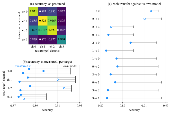
Fig. 6.6(a) is the grid as its script produced it, from the single line imshow(M, cmap=’viridis’, vmin=M.min(), vmax=M.max()). The map is stretched
across the observed range, \(0.875\) to \(0.926\), so the entire excursion from deepest purple to full yellow is \(5.1\) points of accuracy, and no colorbar reports it.
Colorbar
A colormap fitted to the data range, with no colorbar to disclose it, is an error to fix.
Scaling
•vmin=M.min() is the cut baseline of Fig. 7.1(a) moved into color: the scale is pinned to the data rather than to a
meaningful zero, so every apparent difference is inflated by an amount the reader cannot detect. Subtract the reference before you color it!
• Switch the text color on the gray level of the cell rather than on the value.
• Do not re-encode the diagonal, which position already identifies; define every glyph, since an asterisk without a key is a legend without a key.
The comparison the grid is being asked to support is between each transfer and the target channel’s own model, and there are two ways to make it: show that reference, or subtract it. Panels (b) and (c) show it. They
keep the accuracies exactly as they were measured and mark each target’s own model beside them, so the shortfall is a distance on the page rather than a number the script arrived at, and the level of the results survives. That level
is what ch \(3\)’s row is for: a model transferred into ch \(3\) is the least accurate destination of the four, \(0.8772\) against \(0.8928\) into ch \(2\).
Figure 6.6: One \(4 \times 4\) cross-channel record, as it was measured. (a) As produced: viridis stretched over the observed range \(0.875\) to \(0.926\), no colorbar, the diagonal in bold, an unkeyed
asterisk. (b) One row per target channel, three dots in it, one per model transferred in, each joined to the dark rule of that channel’s own model. The segment is the loss the next figure computes, here a length on the page and
nothing else. Ch \(3\)’s whole row, rule included, sits left of the others. (c) The same twelve, sorted and named; the open markers are the three closest transfers. The axis is cut, which points allow and bars do not.
The two panels are not equally successful, and the reason is the reference. Panel (b) draws each of the four references once, so the levels are visible as levels and ch \(3\)’s rule at \(0.900\), against \(0.921\) to
\(0.926\) for the others, is the finding. Panel (c) draws the same four references twelve times, in whatever order the sort produces; and by sorting on the segment it turns the shortfall into a length measured from twelve
different starting points. Sort by a difference only when the marks that carry it start together, which is what a common zero gives and what the next figure draws.
Subtracting the reference is the other way. The quantity the argument turns on is then not the accuracy but the loss against that reference,
where \(a_{ij}\) is the entry of the grid, the accuracy of a classifier trained on channel \(i\) and tested on channel \(j\): the row index \(i\) is the source the model was trained on, the column
index \(j\) is the target it is tested on, and \(a_{jj}\) on the diagonal is the target’s own model, the reference every entry of column \(j\) is measured against. The loss is therefore zero on the diagonal by
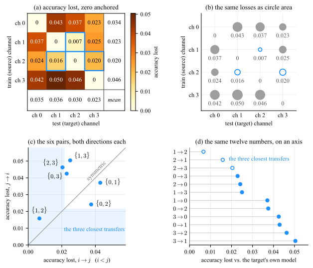
construction. Fig. 6.7(a) draws the same numbers as \(\Delta \), anchored at zero. The row reading survives, the column reading inverts: column \(3\) is the darkest
of Fig. 6.6(a), yet its mean loss of \(0.0228\) is the smallest of the four. What is dark in that column is ch \(3\)’s own model, \(0.900\) against
\(0.921\) to \(0.926\), reported by the raw matrix as though it were the effect. Ch \(3\) is at once the easiest target and the least accurate destination, and it takes both figures to say so: the loss alone cannot state a level,
and the accuracies alone do not isolate the reference.
Figure 6.7: The same record as the loss \(\Delta _{ij}\) of Eq. (6.2), read four ways. (a) The loss anchored at zero, the row and
column means in the margin band. (b) The same layout with the fill replaced by a mark whose area carries the loss and the value printed under it; the three closest transfers are the open rings, and the largest loss is \(7.6\) times
the smallest, which is \(7.6\) times the area of its mark and \(2.7\) times its diameter. (c) One point per pair, its two directions its two coordinates, the lower-indexed source on the horizontal axis; the shaded band holds the three
closest transfers, so a point inside it has a direction among them, and \(\{1,2\}\), inside both arms, transfers well each way. (d) The same twelve losses on a common scale, sorted.
Panel (b) keeps the layout of (a) and changes the mark. The loss becomes the area of a circle, fourth in the ranking of Sec. 6 where shading is sixth, and three
things follow from that alone. No cell is judged against the shade of its neighbors, which is what Sec. 5.2 says a filled grid cannot avoid. An exact zero draws nothing, so
the diagonal empties itself rather than having to be blanked. And the panel needs no colorbar, because the value is printed under every mark, which is what a magnitude channel owes the reader in place of a key. What the area
gives up is precision: the largest loss is \(7.6\) times the smallest, so its mark has \(7.6\) times the area and only \(2.7\) times the diameter, which is the length the eye compares.
Panels (c) and (d) put the same twelve losses at the top of the ranking, as position on a common scale. Panel (c) also answers what a grid invites and no reader performs, whether the relation is symmetric. It is
not.
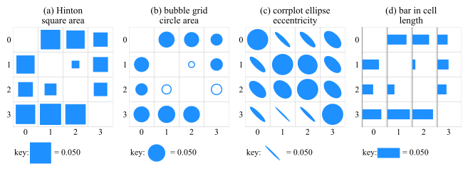
Circle area is not the only mark that frees a cell of its fill. Fig. 6.8 keeps the layout and runs it through four of them. Only length can be ranked by eye.
Every magnitude channel needs a zero and a key
Shading, area and stroke width are all magnitude channels, and each needs a zero the scale is anchored to, and a key on the page stating what one unit of the mark is worth.
Figure 6.8: One matrix of losses, four marks, one cell size, one key per panel. (a) The Hinton diagram, square area, and (b) the bubble grid, circle area, both 4th in the ranking: an exact zero draws nothing, so the
diagonal disappears without being told to, and (b) leaves color free for a second variable, here the three closest transfers. (c) The corrplot ellipse, eccentricity, third, built for a signed bounded quantity, so the largest
mark of the panel lands on the diagonal. Difference between diagonal circiles is indistingushable. (d) The bar in cell, length from a common baseline, second, the only panel that can be ranked by eye. The extremes differ by a factor
of \(7.6\), which is \(7.6\) times the area and \(2.7\) times the side.