Color buys three no other channel offers at the same price:
• it calls attention to one mark among hundreds without enlarging it or moving it,
• it gives a figure something to be remembered by,
• it adds a dimension to a page that has only two.
Color is the easiest channel to misuse
Colors always produce a picture and the picture always looks like data.
5.1 Which part of a color can be ranked
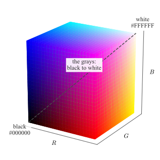
A color in a figure is three numbers: how much red, how much green and how much blue the screen mixes. Each runs from \(0\) to \(1\), or equivalently from \(0\) to \(255\), so every color a figure can use is a point in the box of
Fig. 5.1 — black at the origin where all three are \(0\), white at the opposite corner where all three are \(1\), and the grays on the diagonal between them, where the three
are equal.
Figure 5.1: The RGB cube: every color a figure can use, as a point in the box of the three numbers. The eight corners are black, white and the six pure mixes; the dashed diagonal, where \(R=G=B\), carries the grays from
black to white. The two labeled corners give the three numbers in their usual written form.
Hex codes
The same three numbers are almost always written as six hexadecimal digits, two per channel, running from 00 to FF: #000000 is black, #FFFFFF white, #FF0000
red, #808080 mid gray, and #1F77B4 is the blue matplotlib draws its first line in. Every plotting library, style file and web page accepts this form, and it is the form in which a palette should
be recorded — a color called “blue” is a different color in every tool, while #1F77B4 is not.
Two colors written that way are two points in the cube, so how far apart they are is the straight line between them,
with \(d=0\) for one color written twice and, at the other extreme, \(d=\sqrt {3}\approx 1.73\) for black against white, the diagonal of the cube. Equal steps of \(d\) are not equally visible, so it is a poor measure of
how different two colors look. What it does answer is whether they are distinct at all, which is what a palette of several colors has to guarantee.
What a figure keeps when it is printed in black and white is computable from the three numbers, \(g = 0.21R + 0.72G + 0.07B\), with \(g=0\) for black and \(g=1\) for white. It is called the gray level here. The
approximation is the quantity of interest, because it is what a black-and-white printer or a photocopier actually delivers.
Print it in gray
Any figure may be printed in black and white, projected badly, or photocopied. Test a figure in gray, not draw it in gray.
Dark-to-light ranking
Only dark-to-light can be ranked. Darker and lighter form a scale a reader orders without being told the rule.
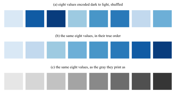
Fig. 5.2 is what that sentence means operationally. Eight values are encoded dark to light and shown three times: shuffled, in their true order, and as the gray a
black-and-white print would keep.
Figure 5.2: Eight values encoded dark to light. (a) Shuffled: the row can be put back in order by eye, without being told which end is large. (b) The true order. (c) The same eight values as the gray a black-and-white print
keeps, falling steadily from \(0.90\) to \(0.21\). Sorting on that gray level recovers the true order exactly, which is the same operation the reader performs in (a).
An ordered quantity therefore needs an ordered channel. If the reader must rank, compare or interpolate, the value has to move the marks from dark to light; if the reader must only tell one thing from another, a different color is
exactly the right answer.
5.2 Color and grayscale are judged in context
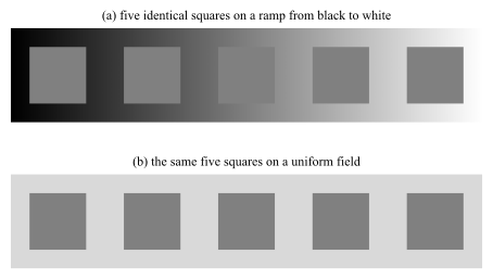
The eye does not measure a color, it compares one. Every patch is reported relative to what surrounds it, so the same ink can be read as two different quantities in two places on the same page. Fig. 5.3 is the demonstration, and it uses no color at all.
Figure 5.3: Gray in context. (a) Five squares, every one of them painted the identical \(\mathrm {RGB}=(0.50,0.50,0.50)\), placed along a ramp running from black to white. They appear to darken steadily from left to
right, and the third square, which sits exactly where the ramp reaches its own value, disappears. (b) The same five squares on a uniform field, where they are visibly one color; the only thing that differed between them in (a) is what
lay behind them, which runs from \(0.10\) to \(0.90\).
Gray is a poor default rather than a safe one (Fig. 5.3).
A shade is only comparable to another shade on the same background.
5.3 Colormaps
Goal: What color for this number?
Colormap
A colormap is a function from a scalar to a color, \(m:[0,1]\to (R,G,B)\), applied after the data has been normalized onto \([0,1]\).
What separates one colormap from another is how the gray level \(g\) of Sec. 5.1 runs along the map, from one end to the other, and the requirement follows from
what the map is being asked to encode. A sequential map has to get lighter throughout, because the reader must be able to rank any two values it produces. A diverging map has to turn exactly once, at the value its center is
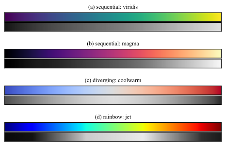
pinned to, which is what makes it read as a distance from that center. A map that turns anywhere else puts an edge on the page where the data has none. Fig. 5.4 shows
four maps against that requirement.
Figure 5.4: Four colormaps, each as the reader sees it and as the gray it prints as. (a) viridis and (b) magma get lighter throughout, over \(0.08\) to \(0.87\) and \(0.00\) to \(0.97\), so either
can carry a magnitude. (c) coolwarm is lightest in the middle and darkens to both ends, which is the center it is built around and not a fault. (d) jet covers \(0.04\) to \(0.92\) and does neither: it is
lightest near the middle, dark at both ends, and reverses on the way.
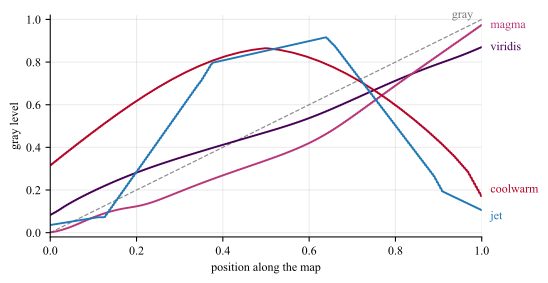
The gray rows are hard to compare bar against bar, so Fig. 5.5 draws the same four gray levels as curves, one against the other.
Figure 5.5: The gray level of the four maps of Fig. 5.4, against position along the map, with the gray map itself as the dashed straight line.
viridis and magma climb without turning. coolwarm turns once, at position \(0.50\). jet turns three times, the last at \(0.64\), after which it darkens again toward its own
maximum. The steps are also uneven, measured as \(\mathrm {std}\lvert \Delta g\rvert / \mathrm {mean}\lvert \Delta g\rvert \) along the map: \(0.20\) for viridis against \(0.69\) for jet,
so equal steps in the data do not arrive as equal steps of gray on the page.
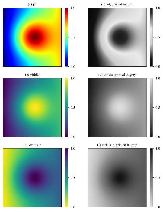
The rainbow colormaps, of which jet is the most common, fail this test outright. Fig. 5.6 shows what the failure does to a field, by reducing each map to the
gray it prints as.
Figure 5.6: Three colormaps, each shown in color and as the gray a black-and-white print leaves. (a) and (b): jet, turns around three times on the way, so the peak comes out dark and a bright false ring
appears around it. (c) and (d): viridis, which only ever gets lighter over the same range. (e) and (f): viridis_r, the same map run backwards, which never stops getting darker and is therefore
just as rankable, with the peak now the darkest ink on the page. Every panel carries its own colorbar, over a field normalized to \([0,1]\), and the bar of a gray panel is the gray that map prints as: the bar of (b) is dark at both
ends and light in the middle, where those of (d) and (f) run one way from end to end.
The dark blob in Fig. 5.6(b) is at the maximum of the field. That inversion, and the bright ring the eye reads as a boundary, are artifacts of the colormap, not features of
the data. A map such as viridis, magma or cividis avoids them by construction: it is built so that equal steps in the data look like equal steps to the reader, and so that it never stops
getting lighter.
jet colormap
Why, then, is it still everywhere? Almost never because anyone chose it.
• Was the MATLAB default until R2014b and the matplotlib default until version 2.0, so every script and every figure written before those releases is jet by
omission, and copied code carries the choice forward without ever restating it.
• Instrument software keeps it alive on its own: spectrum analyzers, thermal cameras, Doppler ultrasound, and seismic and weather displays ship it, often with no setting to change it.
• When a field has trained its readers on a fixed color-to-meaning mapping, or a figure must sit beside an archive drawn the same way, changing the map breaks the comparison the figure exists
to support.
• The three turns of Fig. 5.5 put visible bands and edges on the image, and in color, at full brightness, that extra structure reads
as detail rather than as damage; the author sees a sharp picture, and only the reader of the printed version sees Fig. 5.6(b).
• Color also names a value well even though it ranks values badly. “The red region” is easy to say and easy to match against a colorbar, so reading one value off the figure feels accurate.
Inherited, not chosen
jet on a figure is almost always a default nobody revisited. Change it, unless the figure has to be read against an archive drawn the same way, and (optionaly) say so in the caption.
5.4 Schemes
Goal: Which colors for these categories?
Scheme
A scheme, or palette, is a short fixed list of colors chosen as a set, \(\{c_1,\dots ,c_k\}\).
Colormaps and schemes are convertible, which is why the words get swapped: sampling a colormap at \(k\) points produces a scheme, and interpolating between the entries of a scheme produces a colormap. The first direction is
routine for the ordered families below, and is how most sequential schemes are obtained. The second is not, because interpolating between unordered categories produces colors that stand for nothing.
5.4.1 Choosing a scheme
•Sequential, one color running light to dark, for a quantity with a low end and a high end: counts, magnitudes, probabilities, densities. Its \(k\) colors are a sequential colormap cut
into \(k\) classes.
•Diverging, two colors meeting at a neutral middle, for a quantity with a meaningful center: residuals and errors around zero, correlations, differences between two models. The
middle must be pinned to the meaningful value, or the map asserts a center where none exists.
•Qualitative, different colors of similar darkness, for unordered categories: class labels, model names, cluster identities. Six to eight is the practical ceiling; past that, the colors stop
being distinguishable and direct labeling is the answer.
An excellent source of schemes is Cynthia Brewer’s picker at https://colorbrewer2.org, most of which ships with matplotlib under the same
names.2
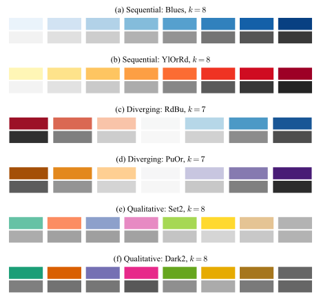
Fig. 5.7 shows two schemes from each family with its gray beneath, which turns the choice from a matter of taste into a matter of shape.
Figure 5.7: Two ColorBrewer schemes from each family, each drawn as the \(k\) fixed colors it is, in color and as the gray it prints as. (a) and (b) Sequential, \(k=8\): the gray only ever moves one way. (c) and (d) Diverging,
\(k=7\), an odd count so that the neutral class is a color of its own rather than a boundary between two: the gray is lightest at that middle class, at position \(0.50\) of the map in both, and darkens to both ends, so the scheme
reads as a distance from a center. (e) and (f) Qualitative, \(k=8\): the gray is deliberately almost flat, so the categories separate by color and none of them looks larger than another.
The gray rows also say what each family must not be used for. A sequential map has no center to put a zero on; a diverging map applied to a quantity with no meaningful center asserts one; and a qualitative map used for a
magnitude leaves the reader nothing to rank with.
2 M. Harrower and C. A. Brewer, “ColorBrewer.org: An Online Tool for Selecting Colour Schemes for
Maps”, The Cartographic Journal, vol. 40, no. 1, 2003, pp. 27–37. The tool also filters on colorblind-safe, print-safe and photocopy-safe, which is the check of Sec. 5.5 applied before the figure exists rather than after.
5.5 Color deficiency
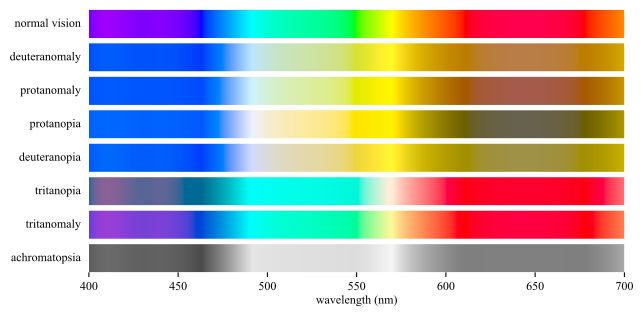
The deficiency is not one condition. Fig. 5.8 passes the visible spectrum through each common form, and Table 5.1
gives how frequent each one is.
Figure 5.8: The visible spectrum as each common form of color vision deficiency receives it. The bar approximates the spectrum and is not a colorimetric reference.
Table 5.1: How common each form is, among people of Northern European ancestry, in the row order of Fig. 5.8. The red-green forms of the first four rows reach
about \(8\%\) of men, two orders of magnitude above the blue-yellow forms below them.
.
Form
Men (%)
Women (%)
Deuteranomaly
5
0.35
Protanomaly
1.3
0.02
Protanopia
1.3
0.02
Deuteranopia
1.2
0.01
Tritanopia
0.008
0.008
Tritanomaly
0.0001
0.0001
Red-green pair
Never let a red-green pair be the only thing separating two series.
Red-green deficiency affects roughly \(8\%\) of men of Northern European ancestry and \(0.4\%\) of women.
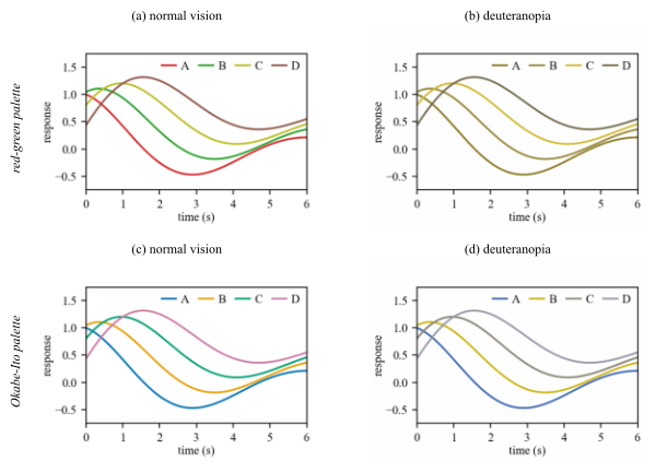
Fig. 5.9 runs the same simulation on one chart drawn with two palettes.3 The data, the layout and the legend are identical in
the two rows, so whatever separates them is the palette alone.
Figure 5.9: One four-series chart under two palettes, each shown in normal vision and under simulated deuteranopia. (c) Okabe-Ito palette. (d) all four series stay separable.
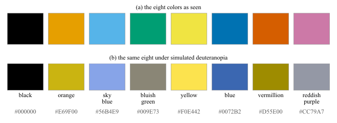
The palette of the lower row is not an invention of that figure. Fig. 5.10 gives it in full: eight colors chosen so that no two of them merge under any common form of
deficiency, published with a name and a code for each so that a figure can be specified in them.
Figure 5.10: The Okabe-Ito qualitative palette, with the name and the hex code of every color. (a) As seen. (b) The same eight under simulated deuteranopia. The closest pair of (a), orange and vermillion, separates by
\(0.263\) in RGB; the closest pair of (b), bluish green and reddish purple, still separates by \(0.202\), so the eight stay tellable apart. Source: Okabe and Ito, Color Universal Design (2008), tabulated in Wong (2011).
3 Both figures simulate deficiency after Machado, Oliveira and Fernandes, “A Physiologically-based Model for Simulation of Color
Vision Deficiency”, IEEE Trans. Visualization and Computer Graphics, vol. 15, no. 6, 2009, pp. 1291–1298. In Fig. 5.9 it is applied to the
rendered pixels of the chart, so the legend keys degrade exactly as the lines do. Fig. 5.8 redraws “Color blindness” by SyntaxTerror, Public domain, via Wikimedia Commons, and Table 5.1 follows the epidemiology table of Wikipedia contributors, “Color blindness”, Wikipedia, The Free Encyclopedia, revision of 11 August 2026, retrieved 18 August 2026.
Okabe-Ito
Eight colors that survive every common deficiency, in the order they are published: #000000, #E69F00, #56B4E9, #009E73, #F0E442, #0072B2,
#D55E00, #CC79A7. Take them in that order and stop when the figure has enough; four of them are Fig. 5.9(c).
A figure that survives both black and white print and vision deficiency simulation is legible to almost everyone.
Double encoding
Use double encoding whenever a distinction matters: give the series different:
• line styles or markers,
• colors.
5.6 Color Meaning
5.6.1 Social aspects
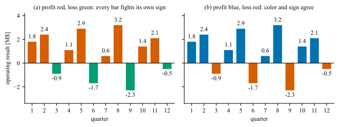
Finally, color carries meaning that the data may not intend. Red reads as loss, danger or failure and green as the opposite, and the reader applies that mapping before reading the axis. A figure that assigns the colors the other way
is not merely unhelpful, it is asserting something about every mark on the page that the numbers contradict. Fig. 5.11 puts one record through both assignments.
Figure 5.11: Twelve quarters of an operating result, drawn twice from the same numbers on the same zero baseline. (a) Profit in red and loss in green: all \(12\) bars carry a color that contradicts their own sign, \(8\) profits
in red and \(4\) losses in green, and the reader has to override the color on every one of them. (b) Profit in blue and loss in red, where none does. The positive side is blue rather than green because red-green is the pair that
roughly \(8\%\) of men cannot separate (Sec. 5.5), so only the negative side keeps the conventional red.
5.6.2 One strong color
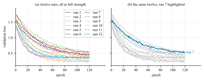
Strong color is a budget. Spend it on the one series, region or mark the text is about, draw everything else in gray at \(20\) to \(40\%\) ink, and let the reader find the subject pre-attentively, by the mechanism of Fig. 4.2, without being told where to look. Fig. 5.12 spends the budget both ways.
Figure 5.12: Twelve validation curves on identical axes. (a) All twelve at full strength, and \(12\) legend keys are needed to name them. (b) Eleven dropped to gray \(0.72\), which is \(28\%\) ink, against one at \(0.37\),
or \(63\%\) ink: a contrast of \(0.35\) that makes the highlighted curve the only thing the eye lands on. It is named at its own end, so the panel needs no key at all.